AI-based Materials and Process Simulation I

Week 02 — Ciarlet’s Finite Element · Vandermonde Matrices and Unisolvence · Basix Elements · Lagrange Variants

Kee-Youn Yoo

Process Systems Laboratory
Department of Chemical and Biomolecular Engineering, SeoulTech

Today

Part	Topic	Time
Quiz	Week 1 material (closed-AI)	10 min
A	Theory — Ciarlet’s element, nodal basis, Vandermonde matrix, unisolvence, Hermite and Argyris	70 min
B	Basix — creating, inspecting and tabulating elements	40 min
C	Lagrange variants — Lebesgue constants, the Runge function in DOLFINx	35 min
D	LLM pitfalls with elements · assignment	15 min

Lab notebook: W02_lab.ipynb · Assignment: W02_HW2.ipynb (due before Week 3)

Week 1 in one slide

Weak form	\int_\Omega \nabla u_h\cdot\nabla v\,dx = \int_\Omega f v\,dx \quad \forall v\in \mathring V_h
Linear system	K_{ij} = \int_\Omega \nabla\phi_j\cdot\nabla\phi_i\,dx, assembled cell by cell
On each cell	K^{(K)}_{ij} \approx \sum_q w_q\,\nabla\phi_j(X_q)\cdot\nabla\phi_i(X_q)\,\|\det J_K\|

Quadrature gave us X_q, w_q. This week: where do the \phi_i come from?

What exactly is a finite element? (Ciarlet)
How is the basis computed, and when does it exist? (Vandermonde, unisolvence)
How does Basix store and evaluate it? (create_element, tabulate)
Where should the nodes be? (Lagrange variants)

Part A — Ciarlet’s Finite Element

§A1 The definition

Definition (Ciarlet, 1978) — Finite element

A finite element is a triple (K, \mathcal{P}, \mathcal{N}):

K\subset\mathbb{R}^d — a bounded closed cell (interval, triangle, tetrahedron, …)
\mathcal{P} — a finite-dimensional space of shape functions on K (usually polynomials)
\mathcal{N}=\{N_0,\dots,N_{n-1}\} — a basis of the dual space \mathcal{P}': the nodal variables (DOFs)

Each N_i:\mathcal{P}\to\mathbb{R} is a linear functional. Examples:

Nodal variable	Formula	Used by
point evaluation	N(p)=p(x_i)	Lagrange
derivative evaluation	N(p)=\partial p/\partial x_j\,(x_i)	Hermite, Argyris
normal derivative	N(p)=\nabla p(x_i)\cdot n	Argyris
integral moment	N(p)=\int_K p\,q\,dx	integral DOFs, bubbles
normal component	N(\mathbf p)=\mathbf p(x_i)\cdot n	Raviart–Thomas (Course II)

§A2 The nodal basis

Definition — Nodal basis

The nodal basis \{\phi_0,\dots,\phi_{n-1}\} of \mathcal{P} is dual to \mathcal{N}: N_i(\phi_j)=\delta_{ij}.

Consequence: every p\in\mathcal{P} is reconstructed from its DOF values, p=\sum_j N_j(p)\,\phi_j . This is why the coefficient vector \mathbf u in K\mathbf u=\mathbf f holds DOF values.

1D Lagrange, degree k: K=[a,b], \mathcal{P}=\mathcal{P}_k, N_i(p)=p(x_i), x_i=a+(b-a)\,i/k: \phi_i(x)=\prod_{j\ne i}\frac{x-x_j}{x_i-x_j}. For other nodal variables there is no such formula. We need a general recipe.

§A3 The Vandermonde matrix

Pick any basis \{\psi_0,\dots,\psi_{n-1}\} of \mathcal{P} (for example monomials).

Definition — Vandermonde matrix

V_{ij}=N_j(\psi_i)

Lemma — Basis transformation

Write \phi_i=\sum_j \mu_{ij}\psi_j. Then \mu=V^{-1}.

Proof. \delta_{ij}=N_j(\phi_i)=\sum_l\mu_{il}N_j(\psi_l)=\sum_l\mu_{il}V_{lj}=(\mu V)_{ij}. \square

Recipe: choose \psi → build V → solve for \mu → \phi_i=\sum_j\mu_{ij}\psi_j. It works for any kind of nodal variable, as long as V is invertible.

§A4 Worked example — two elements on [0,1], same \mathcal{P}_2

\psi=\{1,x,x^2\}

Lagrange: N=\{p(0),\,p(\tfrac12),\,p(1)\} V=\begin{bmatrix}1&1&1\\0&\tfrac12&1\\0&\tfrac14&1\end{bmatrix},\quad \begin{aligned}\phi_0&=1-3x+2x^2\\ \phi_1&=4x-4x^2\\ \phi_2&=-x+2x^2\end{aligned}

Integral DOF: N=\{p(0),\,p(1),\,\int_0^1p\} V=\begin{bmatrix}1&1&1\\0&1&\tfrac12\\0&1&\tfrac13\end{bmatrix},\quad \begin{aligned}\phi_0&=1-4x+3x^2\\ \phi_1&=-2x+3x^2\\ \phi_2&=6x-6x^2\end{aligned}

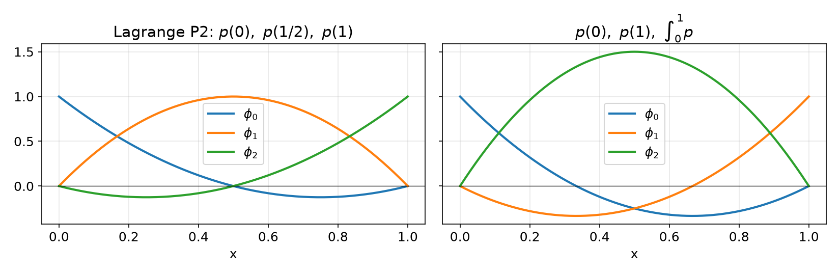
Same space \mathcal{P}_2, different elements: the basis depends on \mathcal N. Check: \int_0^1\phi_2=1, \int_0^1\phi_0=\int_0^1\phi_1=0.

§A5 Unisolvence

When is (K,\mathcal{P},\mathcal{N}) a valid element? \mathcal N must be a basis of \mathcal P'.

Lemma — Equivalent conditions (with \dim\mathcal P=|\mathcal N|=n)

\mathcal N is a basis of \mathcal P'
the Vandermonde matrix V is invertible
if v\in\mathcal P and N_i(v)=0 for all i, then v\equiv 0

Definition — Unisolvence

If (3) holds, \mathcal N determines \mathcal P; the element is unisolvent.

(2)⇔(3): V^T\mathbf c=0 means N_j(\sum_i c_i\psi_i)=0 for all j. A nonzero \mathbf c gives a nonzero v with all DOFs zero.
Always check the count |\mathcal N|=\dim\mathcal P first. Then condition (3) is usually the easiest to prove.
Counterexample: P1 on a “triangle” whose three vertices are collinear. The linear function vanishing on that line has all DOFs zero, so the element is not unisolvent.

§A6 Proving unisolvence — 1D, and a tool for 2D

1D Lagrange, degree k. v\in\mathcal P_k vanishes at k+1 distinct points ⇒ v\equiv0. \square

In 2D a polynomial can vanish at infinitely many points without being zero. We need:

Lemma — Vanishing on a hyperplane

Let p\in\mathcal P_k(\mathbb R^d), k\ge1, vanish on the hyperplane \Pi_L=\{x: L(x)=0\} of a non-degenerate affine L. Then p=L\,q with q\in\mathcal P_{k-1}.

Strategy on a triangle with edge lines L_1,L_2,L_3=0:

p restricted to an edge is a 1D polynomial of degree k. If it vanishes at k+1 edge nodes, it vanishes on the whole edge line.
Factor out L_1, then L_2, then L_3.
What remains must vanish at the interior nodes. Use induction.

§A7 Lagrange elements on triangles

Definition — Pk Lagrange element

K: triangle z_1,z_2,z_3; \mathcal P=\mathcal P_k, \dim=\binom{k+2}{2}; N_{ij}(v)=v(x_{ij}), x_{ij}=z_1+(z_2-z_1)\tfrac ik+(z_3-z_1)\tfrac jk, 0\le j\le i\le k

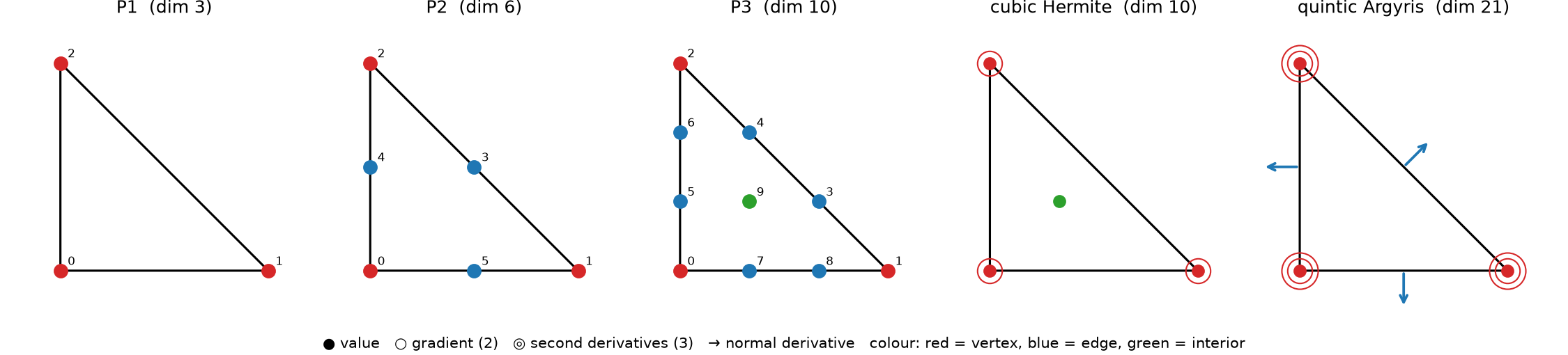
Numbers in the figure = Basix local DOF order: vertices, then edges, then interior. Edge i is opposite vertex i.

	vertex	edge	interior	total
P1	3	0	0	3
P2	3	3	0	6
P3	3	6	1	10
Pk	3	3(k-1)	\binom{k-1}{2}	\binom{k+2}{2}

§A8 Unisolvence of P1 and P2

P1. Let p\in\mathcal P_1 vanish at z_1,z_2,z_3.

On the line \Pi_1 through z_2,z_3, p is linear and vanishes twice, so p=0 on \Pi_1. Hence p=c\,L_1.
0=p(z_1)=c\,L_1(z_1), and L_1(z_1)\ne0, so c=0. \square

P2. Let p\in\mathcal P_2 vanish at the 3 vertices and 3 edge midpoints.

On edge 1, p is quadratic with 3 zeros, so p=L_1Q_1 with Q_1\in\mathcal P_1.
On edge 2, L_1\ne0 except at one vertex. So Q_1 vanishes at 2 points of \Pi_2, Q_1=0 on \Pi_2, and p=c\,L_1L_2.
At the midpoint of edge 3, L_1L_2\ne0, so c=0. \square

Pk, k\ge4 — induction in steps of 3. Factor out L_1L_2L_3; the rest is Q_3\in\mathcal P_{k-3}. Q_3 vanishes on the interior nodes, which form a P(k-3) lattice. Base cases k=1,2,3. You will do P3 in HW2.

§A9 Beyond point values — Hermite and Argyris

Cubic Hermite (triangle)

\mathcal P_3, \dim=10:

value at the 3 vertices (3)
gradient at the 3 vertices (6)
value at the centroid (1)

Quintic Argyris (triangle)

\mathcal P_5, \dim=21:

value at the 3 vertices (3)
gradient at the 3 vertices (6)
all second derivatives at the 3 vertices (9)
normal derivative at the 3 edge midpoints (3)

Both are unisolvent. The proof uses the same tool, with derivative conditions forcing double zeros on edges.
Why would anyone want derivative DOFs? Fourth-order problems (plates, Cahn–Hilliard in primal form) need C^1 continuity across cells.
Which of the two actually gives a C^1 space? It comes down to counting conditions along one edge. You will check it numerically in HW2 Q4.

Part B — Elements in Basix

§B1 Creating and inspecting an element

import basix
P, T, LV = basix.ElementFamily.P, basix.CellType.triangle, basix.LagrangeVariant
e = basix.create_element(P, T, 2, LV.equispaced)
e.dim              # 6
e.points           # [[0,0],[1,0],[0,1],[0.5,0.5],[0,0.5],[0.5,0]]  ← nodes, Basix order
e.entity_dofs      # [[[0],[1],[2]], [[3],[4],[5]], [[]]]           ← by vertex / edge / cell

Fact (Basix 0.11)	Consequence
Degree ≥ 3 Lagrange needs a variant	`create_element(P, T, 3)` → `RuntimeError: ... need to be given a variant`
Degree ≤ 2 without a variant	silently uses `gll_warped`, which equals equispaced for k\le2
DOLFINx `("Lagrange", k)`	uses `gll_warped` for every k
Vertices come first	P2 on the interval: `points` = `[0, 1, 0.5]`, not `[0, 0.5, 1]`

From a DOLFINx space: V.element.basix_element, or V.ufl_element() for the UFL wrapper.

§B2 Tabulation

T_{qj}=\phi_j(X_q) and its derivatives, at any set of reference points:

pts, wts = basix.make_quadrature(T, 4)        # 6 points
tab = e.tabulate(1, pts)                       # derivatives up to order 1
tab.shape                                      # (3, 6, 6, 1)
phi, dphi_dx, dphi_dy = tab[0, :, :, 0], tab[1, :, :, 0], tab[2, :, :, 0]

Axis	Size	Meaning
0	\binom{n_d+d}{d}	derivative: 1; \partial_x,\partial_y; \partial_{xx},\partial_{xy},\partial_{yy}; …
1	n_{pts}	point X_q
2	n_{dofs}	basis function \phi_j
3	value size	1 for scalar elements

Two free sanity checks for any Lagrange element: \sum_j\phi_j\equiv1 and \sum_j\nabla\phi_j\equiv0 (constants are in \mathcal P). For P3 at 4000 lattice points: \max|\sum_j\phi_j-1| = 1.0\times10^{-15}.

§B3 What Basix stores — and why not monomials

Basix stores \phi_i=\sum_j C_{ij}P_j, where \{P_j\} is an orthonormal polynomial basis on the reference cell (Legendre on intervals, Dubiner on triangles).

C = e.coefficient_matrix                  # (6, 6)
Pj = basix.tabulate_polynomials(
    basix.PolynomialType.legendre, T, 2, pts)
np.abs(e.tabulate(0, pts)[0, :, :, 0] - (C @ Pj).T).max()   # 0.0

coefficient_matrix is not V^{-1} in the monomial basis. Several older tutorials say it is.

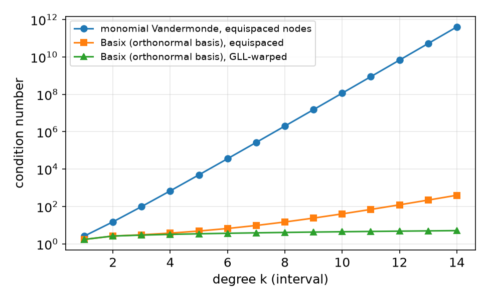
k	monomial V	Basix, GLL
4	6.9\times10^{2}	3.2
8	2.0\times10^{6}	4.1
12	6.8\times10^{9}	4.8

§B4 Math → Basix

Concept	Theory	Basix 0.11
cell K	reference cell	`basix.CellType.triangle`
element (K,\mathcal P,\mathcal N)	Ciarlet triple	`basix.create_element(family, cell, k, variant)`
\dim\mathcal P	\binom{k+2}{2}	`e.dim`
nodes x_i (Lagrange)	N_i(p)=p(x_i)	`e.points`
geometric decomposition	DOFs per vertex/edge/cell	`e.entity_dofs`
\mu=V^{-1}	basis coefficients	`e.coefficient_matrix` (orthonormal basis!)
\phi_j(X_q), \nabla\phi_j(X_q)	tabulation	`e.tabulate(n, pts)` → `(·, npts, ndofs, vs)`
Hermite	value + gradient DOFs	`basix.create_element(basix.ElementFamily.Hermite, T, 3)`
in a DOLFINx space		`basix.ufl.element(P, msh.basix_cell(), k, variant)`

Part C — Where Should the Nodes Be?

§C1 The Lebesgue constant

Interpolation I_k g=\sum_i g(x_i)\phi_i. For any p\in\mathcal P_k, I_kp=p, so \|g-I_kg\|_\infty\le\big(1+\Lambda_k\big)\inf_{p\in\mathcal P_k}\|g-p\|_\infty,\qquad \Lambda_k=\max_{x\in K}\sum_i|\phi_i(x)|.

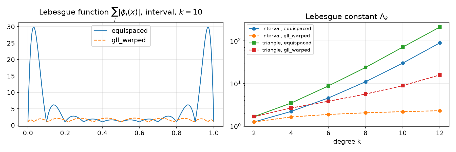
k	interval equi	interval GLL	triangle equi	triangle GLL
4	2.2	1.6	3.5	2.7
8	10.9	2.0	23.6	5.6
12	89.3	2.3	210	15.8

(triangle: max over a 60-division lattice)

Equispaced nodes: \Lambda_k grows exponentially. GLL-warped nodes: \Lambda_k grows slowly (1.25 → 2.29 from k=2 to 12 on the interval).

§C2 Demo — the Runge function in DOLFINx

import basix, basix.ufl
msh = mesh.create_interval(comm, 1, [-1.0, 1.0])           # ONE cell, high degree
el = basix.ufl.element(basix.ElementFamily.P, msh.basix_cell(), 12, basix.LagrangeVariant.equispaced)
V = fem.functionspace(msh, el)
u = fem.Function(V); u.interpolate(lambda x: 1 / (1 + 25 * x[0]**2))

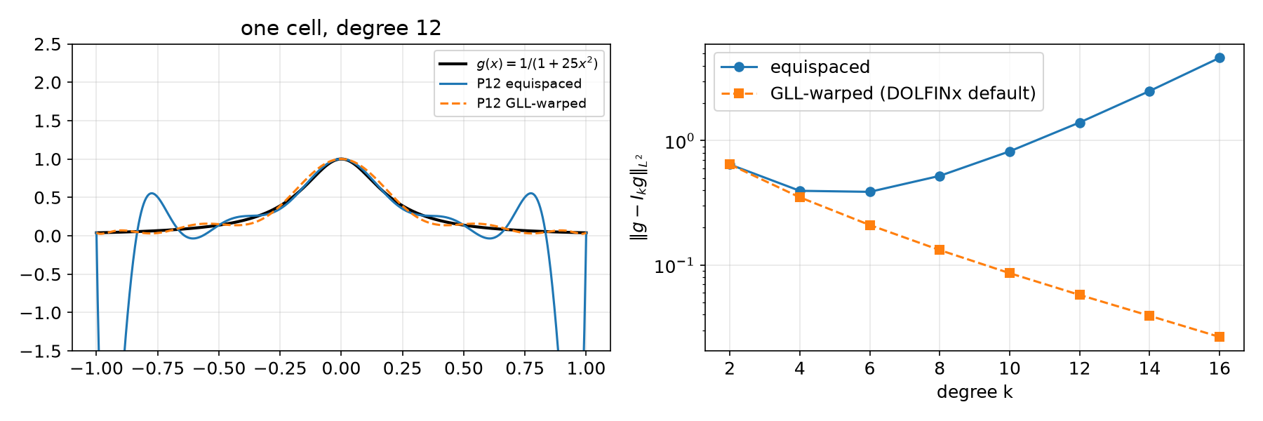
k	equispaced	GLL-warped
4	0.40	0.35
8	0.52	0.13
12	1.40	0.058
16	4.63	0.027

L^2 interpolation error

§C3 Does this matter for you?

P1, P2: all variants coincide. Nothing changes.
P3–P5 (typical high-order work): the differences are small but real. The default gll_warped is the safe choice.
p-methods, spectral elements, k\ge 6: the node choice matters a great deal, for interpolation and for the conditioning of the matrices.
When reading old code: legacy FEniCS used equispaced nodes. The same “P3” can give slightly different numbers in DOLFINx 0.11.

You can see the variant in V.ufl_element().lagrange_variant. Print it whenever results must be reproduced exactly.

Part D — LLMs and Finite Elements · Assignment

§D1 Where LLM-generated element code goes wrong

Kind	Typical examples	Detection
Stale API	Lagrange elements of degree ≥ 3 created without a variant; `ufl.FiniteElement` / `ufl.VectorElement` (removed from UFL); `"CG"` family name (deprecated)	the error message + API sheet
Shape confusion	dropping or misreading an axis of `tabulate` output; `(npts, ndofs)` vs `(ndofs, npts)`	print shapes; \sum_j\phi_j=1
Ordering assumptions	assuming nodes in lexicographic order (`[0, 0.5, 1]`); assuming edge i joins vertices i and i+1	compare with `e.points` / `e.entity_dofs`
Wrong meaning	treating `coefficient_matrix` as the monomial V^{-1}; trusting element metadata or a docstring without testing it	evaluate the claim at points: compare with `tabulate`

The universal check for element code: N_i(\phi_j)=\delta_{ij}, evaluated numerically with your own nodal variables.

Assignment — HW2, due before the Week 3 lecture

HW2 — Unisolvence and nodal bases (100)

Q1 proofs: an integral-DOF element, P3 on a triangle, 1D cubic Hermite (25)
Q2 your own Vandermonde code for Pk on a triangle, compared with Basix; basis plots; what happens at high degree (25)
Q3 when unisolvence fails: six nodes on a circle (20)
Q4 LLM-assisted: the cubic Hermite triangle and the question of C^1 continuity (30)

Submit the executed .ipynb (restart & run all) with the AI-usage log.

Reminder: an error in a %%fenicsx cell does not stop Run all. Read every output before you submit.

Summary

Concept	Key idea	Basix / DOLFINx
Ciarlet element	(K,\mathcal P,\mathcal N), \mathcal N a basis of \mathcal P'	`create_element(family, cell, k, variant)`
Nodal basis	N_i(\phi_j)=\delta_{ij}	`tabulate`
Vandermonde	V_{ij}=N_j(\psi_i), \mu=V^{-1}	`coefficient_matrix` (orthonormal \psi)
Unisolvence	N_i(v)=0\ \forall i\Rightarrow v=0	V invertible
Lagrange Pk	vertex, edge, interior nodes	`points`, `entity_dofs`
Variants	node placement controls \Lambda_k	`LagrangeVariant.gll_warped` (default)

Next week — from local to global

Geometric decomposition, C^0/C^1 continuity, DG spaces; mesh topology and the DOF map in DOLFINx.