AI-based Materials and Process Simulation I

Week 04 — Interpolation Operators · Sobolev Norms · Averaged Taylor Polynomials and Scaling · Functions, Interpolation and Errors in DOLFINx

Kee-Youn Yoo

Process Systems Laboratory
Department of Chemical and Biomolecular Engineering, SeoulTech

Today

Part	Topic	Time
Quiz	Week 3 material (closed-AI)	10 min
A	Theory — interpolation operators, H^k norms, Sobolev embedding, averaged Taylor polynomials, scaling, the error estimate	70 min
B	`fem.Function` and the ways to interpolate in DOLFINx	35 min
C	Measuring errors, convergence rates, interpolation and I/O	40 min
D	LLM pitfalls with functions and norms · assignment	15 min

Lab notebook: W04_lab.ipynb · Assignment: W04_HW4.ipynb (due before Week 5)

Week 3 in one slide

Global space	cells share the DOFs of shared vertices and edges → C^0 (Lagrange)
Dimension	\dim V_h=\sum_d n_d m_d, e.g. (kN+1)^2 for Pk on N\times N
Cell-node map	M(c,i); edge DOFs ordered by global vertex numbers for k\ge3
DOLFINx	`topology.connectivity`, `geometry.dofmaps[0]`, `V.dofmap`, owned + ghost

We can now build V_h. This week: how well can V_h approximate a given u?

The simplest approximation: interpolate, u\mapsto\mathcal I_h u
How do we measure the error? (H^k norms)
How fast does it go to zero as h\to0, and what does that depend on? (Taylor + scaling)
How do we do all this in DOLFINx — and get the numbers right?

Part A — Interpolation Theory

§A1 The local interpolation operator

Definition — Local interpolant

For an element (K,\mathcal P,\mathcal N) with nodal basis \{\phi_i\}: \mathcal I_K v=\sum_i N_i(v)\,\phi_i\ \in\mathcal P . For Lagrange elements N_i(v)=v(x_i): \mathcal I_K v is the polynomial that agrees with v at the nodes.

Property	Statement	Why
Linear	\mathcal I_K(\alpha u+v)=\alpha\mathcal I_Ku+\mathcal I_Kv	N_i linear
Nodal	N_i(\mathcal I_Kv)=N_i(v)	N_i(\phi_j)=\delta_{ij}
Preserves \mathcal P	\mathcal I_Kp=p for all p\in\mathcal P	unisolvence: p-\mathcal I_Kp\in\mathcal P has zero DOFs
Projection	\mathcal I_K\mathcal I_K=\mathcal I_K	apply the previous line to p=\mathcal I_Kv

Polynomial preservation is the engine of the whole theory: the error comes only from the part of v that \mathcal P cannot represent.

§A2 The global interpolation operator

Definition — Global interpolant

\mathcal I_h u\in V_h with (\mathcal I_h u)|_K=\mathcal I_K u for every K\in\mathcal T_h.

Well defined and in V_h: neighbouring cells evaluate the same shared DOFs (Week 3, C^0 decomposition), so the pieces match.

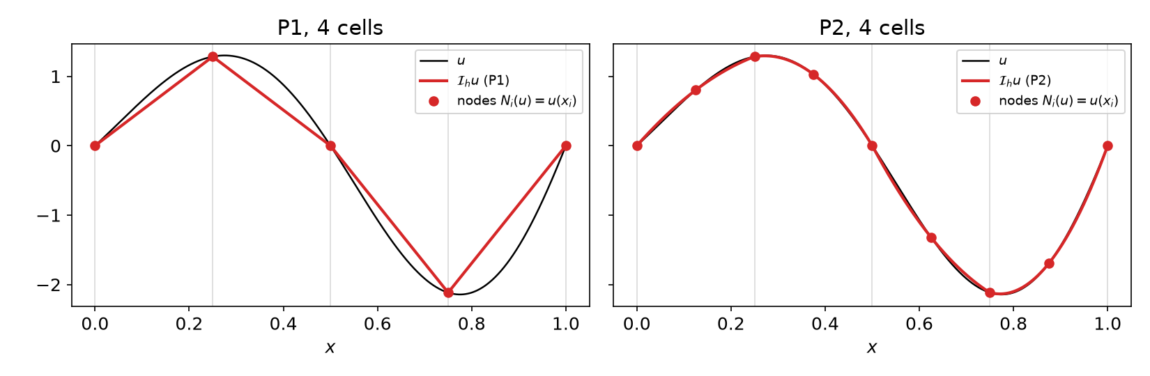
For Lagrange: \mathcal I_h u=\sum_j u(x_j)\,\phi_j — the coefficient vector is just u at the DOF coordinates. That is u_h.interpolate(...).

§A3 Sobolev norms

Multi-index \alpha=(\alpha_1,\dots,\alpha_n), |\alpha|=\sum\alpha_i, D^\alpha u=\partial^{|\alpha|}u/\partial x_1^{\alpha_1}\cdots\partial x_n^{\alpha_n}.

Definition — H^k seminorm and norm

|u|_{H^k(\Omega)}^2=\sum_{|\alpha|=k}\int_\Omega|D^\alpha u|^2\,dx,\qquad \|u\|_{H^k(\Omega)}^2=\sum_{j=0}^k|u|_{H^j(\Omega)}^2 . H^k(\Omega) = functions with finite \|\cdot\|_{H^k} (derivatives in the weak sense — Week 7).

	written out	in UFL
\\|e\\|_{L^2}=\\|e\\|_{H^0}	\left(\int e^2\right)^{1/2}	`inner(e, e) * dx`
\|e\|_{H^1}	\left(\int\|\nabla e\|^2\right)^{1/2}	`inner(grad(e), grad(e)) * dx`
\|e\|_{H^2}	\left(\sum_{i,j}\int(\partial_{ij}e)^2\right)^{1/2}	`inner(grad(grad(e)), grad(grad(e))) * dx`

The seminorm vanishes on polynomials of degree <k: |p|_{H^{k}}=0 for p\in\mathcal P_{k-1}.

§A4 When is \mathcal I_h defined? — Sobolev embedding

Lagrange DOFs are point values. Is u(x_i) meaningful for u\in H^k?

Theorem — Sobolev embedding

If \Omega\subset\mathbb R^n is Lipschitz and k>n/2, then \max_{\bar\Omega}|u|\le C\,\|u\|_{H^k(\Omega)} (and u is continuous).

	n=1	n=2	n=3
point values bounded for	H^1	H^2	H^2

In 2D, H^1 is not enough. u(x)=\log\bigl|\log|x|\bigr| on |x|<1/e has \int|\nabla u|^2<\infty but u(0)=\infty. So the estimates below assume u\in H^{k+1} with k+1\ge2, and Lagrange interpolation of a merely H^1 function is not defined. (Other “interpolants” — Clément, Scott–Zhang — average instead of evaluating.)

§A5 Averaged Taylor polynomials

A Taylor polynomial at one point needs pointwise derivatives. Averaging over a ball B gives an integral-friendly version.

Definition — Averaged Taylor polynomial

K star-shaped w.r.t. a ball B, cut-off \varphi\ge0 supported in B with \int\varphi=1: Q_k u(x)=\int_B T^k_y u(x)\,\varphi(y)\,dy,\qquad T^k_yu(x)=\sum_{|\alpha|\le k}\frac{D^\alpha u(y)}{\alpha!}(x-y)^\alpha .

Q_k u\in\mathcal P_k, and Q_kp=p for p\in\mathcal P_k.
D^\alpha Q_k u=Q_{k-|\alpha|}D^\alpha u — averaging and differentiation commute.

Theorem — Bramble–Hilbert (Taylor remainder)

On K with diameter d, for 0\le i\le k+1: \;|u-Q_ku|_{H^i(K)}\le C\,d^{\,k+1-i}\,|u|_{H^{k+1}(K)}, with C depending on k, n and the ratio d/\rho_B.

Only the (k+1)-th derivatives of u appear: lower-order parts are reproduced exactly.

§A6 The estimate on the reference cell

Lemma — Reference-cell estimate

On the reference triangle \hat K, for Pk Lagrange (k\ge1) and 0\le i\le k+1: \;|\hat u-\hat{\mathcal I}\hat u|_{H^i(\hat K)}\le \hat C\,|\hat u|_{H^{k+1}(\hat K)}.

Proof. Let p=Q_k\hat u\in\mathcal P_k. Polynomial preservation gives \hat{\mathcal I}p=p, so \hat u-\hat{\mathcal I}\hat u=(\hat u-p)-\hat{\mathcal I}(\hat u-p).

\|\hat u-p\|_{H^{k+1}(\hat K)}\le C|\hat u|_{H^{k+1}(\hat K)} (Bramble–Hilbert, all i\le k+1).
\|\hat{\mathcal I}w\|_{H^{k+1}(\hat K)}\le\sum_j|w(\hat x_j)|\,\|\hat\phi_j\|_{H^{k+1}}\le C\max|w|\le C\|w\|_{H^{k+1}(\hat K)} (Sobolev, k+1\ge2>n/2).
Apply 2 to w=\hat u-p and add. \square

Three ingredients: polynomial preservation, bounded DOFs (Sobolev), Taylor remainder.

§A7 Scaling to a physical cell

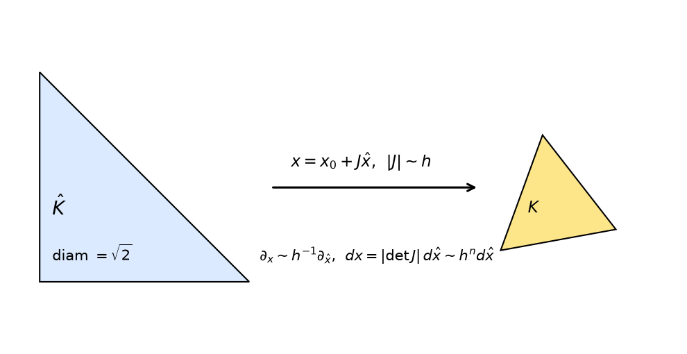
Affine map F_K(\hat x)=x_0+J_K\hat x, \hat v=v\circ F_K. Let h_K=\operatorname{diam}K, \rho_K = diameter of the largest inscribed ball.

Lemma — Scaling of seminorms

|v|_{H^m(K)}\le C\,\|J_K^{-1}\|^m\,|\det J_K|^{1/2}\,|\hat v|_{H^m(\hat K)} and |\hat v|_{H^m(\hat K)}\le C\,\|J_K\|^m\,|\det J_K|^{-1/2}\,|v|_{H^m(K)}, with \|J_K\|\le\dfrac{h_K}{\hat\rho}, \|J_K^{-1}\|\le\dfrac{\hat h}{\rho_K}.

Chain rule (m derivatives → m factors of J) and change of variables (dx=|\det J|\,d\hat x).

For Lagrange elements interpolation commutes with the map: \widehat{\mathcal I_Ku}=\hat{\mathcal I}\hat u (nodes map to nodes).

§A7 Scaling — the proof

\begin{aligned} |u-\mathcal I_Ku|_{H^i(K)} &\le C\,\|J_K^{-1}\|^{i}\,|\det J_K|^{1/2}\;|\hat u-\hat{\mathcal I}\hat u|_{H^i(\hat K)} &&\text{(scale down)}\\ &\le C\,\|J_K^{-1}\|^{i}\,|\det J_K|^{1/2}\;\hat C\,|\hat u|_{H^{k+1}(\hat K)} &&\text{(reference estimate)}\\ &\le C\,\|J_K^{-1}\|^{i}\,\|J_K\|^{k+1}\;|u|_{H^{k+1}(K)} &&\text{(scale up)}\\ &\le C\,\Bigl(\frac{h_K}{\rho_K}\Bigr)^{i}\,h_K^{\,k+1-i}\;|u|_{H^{k+1}(K)} . \end{aligned}

i=0 (L^2): no shape factor at all.
i\ge1: the factor \sigma_K=h_K/\rho_K appears. Shape regularity — \sigma_K\le\sigma for all cells — makes it a constant.
Is shape regularity necessary? Thin triangles are common near walls. → HW4 Q3.

§A8 The global estimate

Theorem — Interpolation error

Shape-regular family \{\mathcal T_h\}, Pk Lagrange, u\in H^{k+1}(\Omega), k\ge1. For i=0,1: |u-\mathcal I_hu|_{H^i(\Omega)}\le C\,h^{\,k+1-i}\,|u|_{H^{k+1}(\Omega)},\qquad h=\max_K h_K .

Proof. Square the local estimate and sum over cells: \sum_K h_K^{2(k+1-i)}|u|^2_{H^{k+1}(K)}\le h^{2(k+1-i)}|u|^2_{H^{k+1}(\Omega)}. \square (i\ge2 is not meaningful for C^0 elements globally — \nabla\mathcal I_hu jumps across edges.)

	\\|u-\mathcal I_hu\\|_{L^2}	\|u-\mathcal I_hu\|_{H^1}
P1	h^2	h
P2	h^3	h^2
P3	h^4	h^3

Why it matters: Céa’s lemma (Week 7) bounds the FE error by the best approximation, and \mathcal I_hu is one candidate: \|u-u_h\|_{H^1}\le C\inf_{v_h}\|u-v_h\|_{H^1}\le C\|u-\mathcal I_hu\|_{H^1}. Interpolation rates are the FE rates.

§A9 When u is not smooth

If u\in H^{s} only, with 1<s<k+1, the same argument (with k replaced by s-1) gives |u-\mathcal I_hu|_{H^i}\le Ch^{\,s-i}|u|_{H^s}. Regularity, not degree, limits the rate.

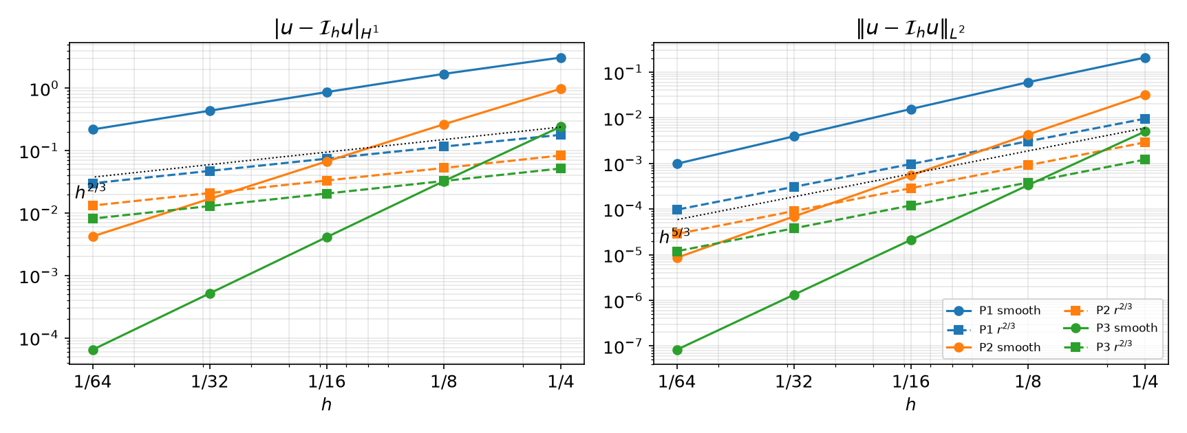
u=r^{2/3}	L^2 rate	H^1 rate
P1	1.66	0.66
P2	1.67	0.67
P3	1.67	0.67

r^{\alpha}\in H^{1+\alpha-\varepsilon} near a 2D corner, so s=5/3: rates 5/3 and 2/3 for every k. Such corner singularities appear in the solutions of PDEs on non-convex domains (L-shapes, re-entrant corners).

Part B — Functions and Interpolation in DOLFINx

§B1 `fem.Function`: a coefficient vector on a space

u_h=\sum_j u_j\,\phi_j\qquad\longleftrightarrow\qquad \texttt{u.x.array}=(u_0,u_1,\dots)

V = fem.functionspace(msh, ("Lagrange", 2))
u = fem.Function(V, name="u")       # all zeros; the name is used in output files
u.x.array                           # NumPy view: owned DOFs first, then ghosts
u.function_space, u.x.index_map, u.x.block_size

4×4 mesh, P2	`-np 1`	`-np 2`, rank 0	`-np 2`, rank 1
`len(u.x.array)`	81	57	57
owned / ghosts	81 / 0	39 / 18	42 / 15

If you write into u.x.array yourself, call u.x.scatter_forward() so ghosts get the owners’ values.
interpolate and solvers do this for you.
Ghost values are copies: never sum over u.x.array to get a global number.

§B2 Interpolating a Python function

u.interpolate(lambda x: np.sin(np.pi * x[0]) * np.cos(np.pi * x[1]))   # x has shape (3, n_points)
w.interpolate(lambda x: np.vstack((x[0], -x[1])))                       # vector space: return (gdim, n_points)

DOLFINx passes the physical coordinates of all interpolation points at once; the callable must be vectorised.

Mistake	What happens (0.11)
`lambda x: 1.0`	`TypeError: interpolate_f(): incompatible function arguments` → use `np.full(x.shape[1], 1.0)`
vector field returned as `(n_points, 2)`	`RuntimeError: Interpolation data has the wrong shape/size.`
`np.sin` applied to a UFL coordinate	`TypeError: loop of ufunc does not support argument 0 of type Indexed…`
`x[0]**0.75`	`nan` at some DOFs: boundary coordinates can be -3\times10^{-18}

NumPy for callables (x is an array); UFL (ufl.sin, ufl.SpatialCoordinate) for forms and fem.Expression.

§B3 Interpolating other things

u1.interpolate(u3)                                    # Function → Function, same mesh (P3 → P1, P1 → P3, …)

expr = fem.Expression(ufl.grad(u3), VD.element.interpolation_points)   # property: no ()
g = fem.Function(VD); g.interpolate(expr)             # any UFL expression, e.g. ∇u into a DG vector space

kappa.interpolate(lambda x: np.full(x.shape[1], 10.0), cells0=right_cells)   # only on some cells

P3 → P1 by interpolate(u3) equals direct P1 interpolation of the same u (difference 4\times10^{-16}): it evaluates u_3 at the P1 nodes.
cells0=: piecewise data, e.g. a DG0 conductivity \kappa=1 / 10 on the two halves of the square (\int\kappa=5.5).

Different meshes need the non-matching version:

cells = np.arange(n_cells_local_plus_ghost, dtype=np.int32)          # target cells
data  = fem.create_interpolation_data(V_coarse, V_fine, cells, padding=1e-14)
u_coarse.interpolate_nonmatching(u_fine, cells, interpolation_data=data)

Plain u_coarse.interpolate(u_fine) → RuntimeError: Meshes do no match. A quadratic moved from a triangle mesh to a quadrilateral mesh with P2 arrives with error 2\times10^{-16} — polynomial preservation again.

Part C — Measuring Errors

§C1 Norms of errors in UFL

x = ufl.SpatialCoordinate(msh)
u_ex = ufl.sin(2 * ufl.pi * x[0]) * ufl.cos(2 * ufl.pi * x[1])      # exact solution as UFL
e = u_h - u_ex

def norm(form):                                                     # parallel-safe
    return np.sqrt(msh.comm.allreduce(fem.assemble_scalar(fem.form(form)), op=MPI.SUM))

L2 = norm(ufl.inner(e, e) * ufl.dx)
H1 = norm(ufl.inner(ufl.grad(e), ufl.grad(e)) * ufl.dx)             # seminorm
rate = np.log(E[i - 1] / E[i]) / np.log(h[i - 1] / h[i])

Pk, u=\sin2\pi x\cos2\pi y	L^2, N=64	rate	H^1, N=64	rate
P1	9.8\times10^{-4}	2.00	2.2\times10^{-1}	1.00
P2	8.6\times10^{-6}	3.00	4.2\times10^{-3}	2.00
P3	8.3\times10^{-8}	4.00	6.5\times10^{-5}	3.00

Rates from N=32\to64; the full table and plot are in §A9.

§C2 Three ways to get a wrong error

1 · The exact solution lives in the same space. Interpolating u_{\rm ex} into V and comparing with \mathcal I_hu: the error is exactly 0 (P1, N=8: 0.0 vs 1.56\times10^{-2} with the UFL expression). Use a UFL expression, or interpolate into a higher-degree space.

2 · Too little quadrature. UFL estimates the degree for sin as degree + 2; forcing a low degree changes the answer:

`quadrature_degree`	1	2	4	8	default (12)
\\|u-\mathcal I_hu\\|_{L^2}	0.0189	0.0146	0.01556	0.015553	0.015553

3 · Forgetting the parallel sum (allreduce), or taking sqrt of a per-rank value. Test with -np 1 and -np 2.

Unit test for every pipeline: polynomial preservation. Interpolating x^2+xy: P1 error 4.4\times10^{-3}; P2, P3 errors 2\times10^{-16}.

§C3 [D] Interpolation and I/O

From the DOLFINx demo Interpolation and IO: a field whose normal component jumps at x=0.5, in an H(\mathrm{curl}) space.

V  = fem.functionspace(msh, ("N1curl", 1))                     # Nédélec: tangential continuity only
u  = fem.Function(V)
u.interpolate(lambda x: np.vstack((x[0], x[1])), cells0)       # cells with x ≤ 0.5
u.interpolate(lambda x: np.vstack((x[0] + 1, x[1])), cells1)   # cells with x ≥ 0.5
V0 = fem.functionspace(msh, ("DG", 1, (2,)))                   # discontinuous Lagrange for output
u0 = fem.Function(V0); u0.interpolate(u)

Just left / right of (0.5, 0.3): u_0=(0.469,\,0.281) and (1.531,\,0.281) — u_x jumps, u_y is continuous.

Writer	What it accepts	Use
`io.XDMFFile`	functions of the same degree as the mesh (P1 on an affine mesh)	P2 → `RuntimeError: Degree of output Function must be same as mesh degree.`
`io.VTXWriter` (ADIOS2)	Lagrange/DG of any degree, time series	open the `.bp` folder in ParaView; check `dolfinx.has_adios2`

On Colab: write to /tmp/fnx/ or Drive, then download and open in ParaView.

§C4 Math → DOLFINx

Math	DOLFINx 0.11
u_h=\sum u_j\phi_j	`u = fem.Function(V)`; `u.x.array` (owned + ghosts)
\mathcal I_hu for a formula u	`u.interpolate(lambda x: ...)` (NumPy, vectorised)
\mathcal I_h of another FE function	`interpolate(v)`; other mesh: `create_interpolation_data` + `interpolate_nonmatching`
\mathcal I_h of an expression (\nabla u, \kappa\nabla u)	`fem.Expression(expr, V.element.interpolation_points)`
piecewise data	`interpolate(f, cells0=cells)`
\\|e\\|_{L^2}, \|e\|_{H^1}	`sqrt(allreduce(assemble_scalar(form(inner(e,e)*dx))))`, same with `grad`
rate	\log(E_{i-1}/E_i)/\log(h_{i-1}/h_i)
output	`VTXWriter` (any order), `XDMFFile` (mesh degree)

Part D — LLMs, Functions and Norms · Assignment

§D1 Where LLM-generated interpolation/error code goes wrong

Kind	What it looks like	Detection
NumPy vs UFL	NumPy functions in forms, UFL objects in callables	the `TypeError`; know which side each object lives on
Shapes	callables that return a scalar, a tuple of the wrong length, or the transposed array	the error message; print `x.shape` inside the callable
Self-fulfilling checks	comparing with a reference that lives in the same space; low quadrature	polynomial preservation; a reference you trust
Stale API	interpolation between meshes, writer classes and their arguments from older versions	the API sheet; read the signature
Parallel	per-rank norms, missing `sqrt`/`allreduce`	`-np 1` = `-np 2`

Before trusting a rate: run a polynomial that must be reproduced exactly, and check that the rate is constant over several refinements.

Assignment — HW4, due before the Week 5 lecture

HW4 — Interpolation convergence rates (100)

Q1 proofs: the 1D estimate by Rolle and scaling; how norms scale (25)
Q2 convergence study: P1–P3, a smooth function and a function singular along an edge; graded meshes (35)
Q3 one-triangle experiment: which triangle shapes are harmful for |u-\mathcal I_hu|_{H^1}? (20)
Q4 LLM-assisted: transfer a P2 field between non-matching meshes, verify, write it out (20)

Submit the executed .ipynb (restart & run all) with the AI-usage log.

Reminder: an error in a %%fenicsx cell does not stop Run all. Read every output before you submit.

Summary

Concept	Key idea	DOLFINx
Interpolant	\mathcal I_Kv=\sum N_i(v)\phi_i, preserves \mathcal P	`interpolate`
H^k norms	\|u\|_{H^k}^2=\sum_{\|\alpha\|=k}\\|D^\alpha u\\|^2	UFL `inner`, `grad`
Sobolev	point values need k>n/2	—
Error estimate	\|u-\mathcal I_hu\|_{H^i}\le Ch^{k+1-i}\|u\|_{H^{k+1}}	rates 2/1, 3/2, 4/3
Ingredients	Taylor remainder + polynomial preservation + scaling	—
Limits	regularity of u; shape of cells	graded meshes; HW4

Next week — Lax–Milgram

Riesz representation, coercivity and continuity, well-posedness of Poisson/Helmholtz; assembly and PETSc KSP; the method of manufactured solutions.