AI-based Materials and Process Simulation I

Week 06 — Boundary Conditions: Mean Estimate · Pure Neumann · Trace Inequality · Partial Dirichlet · Robin · Dirichlet Lifting in DOLFINx · Subdomains, Multi-Material Problems and Gmsh

Kee-Youn Yoo

Process Systems Laboratory
Department of Chemical and Biomolecular Engineering, SeoulTech

Today

Part	Topic	Time
Quiz	Week 5 material (closed-AI)	10 min
A	Theory — weak forms with mixed boundary conditions, mean estimate, pure Neumann, trace inequality, partial Dirichlet, Robin	65 min
B	Dirichlet conditions in DOLFINx — locating DOFs, `dirichletbc`, lifting, the assembly pipeline	35 min
C	Neumann and Robin terms, pure Neumann in PETSc, subdomains, multi-material problems, Gmsh	45 min
D	LLM pitfalls with boundary conditions · assignment	15 min

Lab notebook: W06_lab.ipynb · Assignment: W06_HW6.ipynb (due before Week 7)

Week 5 in one slide

Lax–Milgram	b continuous (M) + coercive (\gamma) on a Hilbert space ⇒ unique u, \\|u\\|\le\\|F\\|_{V'}/\gamma — the same on every V_h
On V_h	\gamma_h=\lambda_{\min}(K,G) with the Gram matrix G=M+K
Helmholtz	M=\gamma=1; Neumann condition is natural
Poisson	b(v,v)=\|v\|^2_{H^1} — a seminorm; \gamma_h\approx0 with natural BCs, 0.952 with u=0 on \partial\Omega
MMS	\tilde u with the BC, f by UFL, rates over ≥ 3 meshes

This week: which boundary conditions remove the constants, and how much of the boundary is enough?

Pure Neumann (mean estimate), partial Dirichlet (trace inequality), Robin
Then the implementation: Dirichlet lifting, boundary markers, nullspaces, subdomains and Gmsh meshes

Part A — Boundary Conditions in the Theory

§A1 Three kinds of boundary conditions

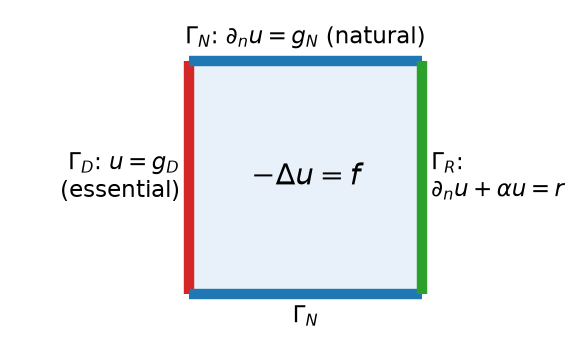
\partial\Omega=\Gamma_D\cup\Gamma_N\cup\Gamma_R, \;\mathbf n = outward unit normal.

Condition	Name	Where it goes
u=g_D on \Gamma_D	essential (Dirichlet)	in the space: u\in g_D+V_D
\partial_nu=g_N on \Gamma_N	natural (Neumann)	in F: \int_{\Gamma_N}g_Nv
\partial_nu+\alpha u=r on \Gamma_R	Robin	in b: \alpha\!\int_{\Gamma_R}\!uv; in F: \int_{\Gamma_R}rv

Robin is the convective (Newton cooling) condition -k\partial_nT=h(T-T_\infty): \alpha=h/k, r=hT_\infty/k. \alpha\to0: Neumann; \alpha\to\infty: Dirichlet u=r/\alpha.

§A2 The weak form with mixed conditions

Multiply -\Delta u=f by v with v=0 on \Gamma_D and integrate by parts: \int_\Omega\nabla u\cdot\nabla v-\int_{\partial\Omega}\partial_nu\,v=\int_\Omega fv .

On \Gamma_D the boundary term vanishes because v=0; on \Gamma_N and \Gamma_R insert the condition:

Weak form

Find u\in H^1(\Omega) with u=g_D on \Gamma_D such that for all v\in V_D=\{v\in H^1(\Omega):v=0\text{ on }\Gamma_D\} \underbrace{\int_\Omega\nabla u\cdot\nabla v+\alpha\int_{\Gamma_R}uv}_{b(u,v)}=\underbrace{\int_\Omega fv+\int_{\Gamma_N}g_Nv+\int_{\Gamma_R}rv}_{F(v)} .

Lifting: write u=u_0+u_g with any u_g\in H^1, u_g=g_D on \Gamma_D. Then u_0\in V_D solves b(u_0,v)=F(v)-b(u_g,v) — a problem on the linear space V_D, where Lax–Milgram applies. Two questions remain: is F bounded (boundary integrals!), and is b coercive on V_D?

§A3 The key inequality

b(v,v)\ge|v|^2_{H^1}, but coercivity needs the full norm \|v\|^2_{H^1}=\|v\|^2_{L^2}+|v|^2_{H^1}. It is enough to have, on the space we work in, \|v\|_{L^2}\le C\,|v|_{H^1}\quad\Longrightarrow\quad \|v\|^2_{H^1}\le(1+C^2)\,|v|^2_{H^1}\le(1+C^2)\,b(v,v),\qquad \gamma=\frac{1}{1+C^2}.

A Poincaré-type inequality. It fails on all of H^1 (v=1), so the space must exclude constants:

Space	What excludes the constants	Tool
\bar V=\{v:\int_\Omega v=0\}	zero mean	mean estimate (§A4)
V_D=\{v:v=0\text{ on }\Gamma_D\}, \|\Gamma_D\|>0	zero on part of the boundary	mean estimate + trace inequality (§A6–A7)
H^1 with Robin, \alpha>0	\alpha\int_{\Gamma_R}v^2 in b	trace inequality (§A9)

On V_h the best constant is again an eigenvalue: C_h^2=\max\frac{\mathbf v^TM\mathbf v}{\mathbf v^TK\mathbf v} over the space =1/\lambda_{\min}.

§A4 The mean estimate

Lemma — mean estimate

For u\in H^1(\Omega) (in particular any C^0 finite element function), \Omega convex, \bar u=\frac1{|\Omega|}\int_\Omega u: \|u-\bar u\|_{L^2(\Omega)}\le C\,|u|_{H^1(\Omega)},\qquad C\text{ depends only on }\Omega .

Proof sketch. u(x)-u(y)=\int_0^1(x-y)\cdot\nabla u(y+s(x-y))\,ds (FE fundamental theorem of calculus on segments). Average over y: u(x)-\bar u=\frac1{|\Omega|}\int_\Omega\!\int_0^1(x-y)\cdot\nabla u(\cdots)\,ds\,dy. Square, Cauchy–Schwarz, split the s-integral at \frac12 and change variables in each half — the same structure as the averaged Taylor polynomial of Week 4. \square

Best constant on the unit square: C=1/\sqrt{\lambda_2}, where \lambda_2=\pi^2 is the first non-zero Neumann eigenvalue of -\Delta (\cos\pi x).

P1, C_h=1/\sqrt{\lambda_2(K,M)}	N=4	N=8	N=16	N=32	limit 1/\pi
	0.3107	0.3163	0.3178	0.3182	0.3183

§A5 Pure Neumann

-\Delta u=f in \Omega, \partial_nu=g on all of \partial\Omega: \;b(u,v)=\int\nabla u\cdot\nabla v, \;F(v)=\int fv+\int_{\partial\Omega}gv.

Compatibility. Take v=1: b(u,1)=0, so a solution exists only if \displaystyle\int_\Omega f+\int_{\partial\Omega}g=0 (sources = outflow).
Non-uniqueness. If u solves, so does u+c. Fix the constant by working in \bar V=\{v:\int v=0\}.

Theorem — pure Neumann

On \bar V (and on \bar V_h=V_h\cap\bar V) b is coercive with \gamma=1/(1+C^2), C from the mean estimate. With compatible data the solution u\in\bar V satisfies b(u,v)=F(v) for all v\in H^1 (split v=(v-\bar v)+\bar v; the constant part gives 0=0).

Unit square: \gamma=\pi^2/(1+\pi^2)=0.908, independent of h. F contains \int_{\partial\Omega}gv — bounded on H^1 only thanks to the trace inequality.

§A6 Trace inequality

Lemma — FE divergence theorem

For a C^1 vector field \boldsymbol\xi and u in a C^0 FE space: \int_\Omega\nabla\cdot(\boldsymbol\xi u)=\int_{\partial\Omega}\boldsymbol\xi\cdot\mathbf n\,u — the interior facet terms cancel because u is continuous and \mathbf n^+=-\mathbf n^-.

Theorem — trace inequality

On a polygon, \;\|u\|_{L^2(\partial\Omega)}\le C_T\,\|u\|_{H^1(\Omega)}.

Proof. Take \boldsymbol\xi with \boldsymbol\xi\cdot\mathbf n=1 on \partial\Omega, apply the lemma to u^2: \int_{\partial\Omega}u^2=\int_\Omega(\nabla\cdot\boldsymbol\xi)u^2+2u\,\boldsymbol\xi\cdot\nabla u\le c\bigl(\|u\|^2_{L^2}+\|u\|_{L^2}|u|_{H^1}\bigr)\le c'\|u\|^2_{H^1} (2ab\le a^2+b^2). \square

P1, C_{T,h}^2=\lambda_{\max}(B,G), B_{ij}=\int_{\partial\Omega}\phi_j\phi_i	N=4	N=8	N=16	N=32
unit square	4.156	4.163	4.165	4.165

Bounded. Compare Week 5 (HW5 Q3): the dual norm of a point value grows like \log(1/h) in 2D. Lines carry H^1 functions; points do not.

§A7 Partial Dirichlet

Theorem — partial Dirichlet (Brenner & Scott)

If \Gamma_D\subset\partial\Omega has positive length, then \|v\|_{L^2}\le C|v|_{H^1} on V_D, so Poisson is coercive on V_D and on V_h\cap V_D, uniformly in h.

Proof. \|v\|_{L^2}\le\|v-\bar v\|_{L^2}+\|\bar v\|_{L^2}. First term: mean estimate. Second: since v=0 on \Gamma_D, \|\bar v\|_{L^2}=\frac{|\Omega|^{1/2}}{|\Gamma_D|}\Bigl|\int_{\Gamma_D}(\bar v-v)\Bigr|\le\frac{|\Omega|^{1/2}}{|\Gamma_D|^{1/2}}\|v-\bar v\|_{L^2(\partial\Omega)}\le\frac{|\Omega|^{1/2}C_T}{|\Gamma_D|^{1/2}}\|v-\bar v\|_{H^1}\le C|v|_{H^1}. \ \square

\gamma_h for \Gamma_D=\{x=0,\ 0\le y\le\ell\} (P1):

\ell	all of \partial\Omega	1 (one side)	1/2	1/4	1/8	1/16
N=16	0.9522	0.7118	0.6283	0.5135	0.4317	0.3767
N=32	0.9519	0.7116	0.6240	0.5069	0.4227	0.3643

Smaller \Gamma_D → smaller \gamma (the constant has |\Gamma_D|^{-1/2}), but for fixed \ell>0 it settles as h\to0.

§A8 A point is not a boundary condition

Shrink \Gamma_D to one DOF (a vertex p with v(p)=0):

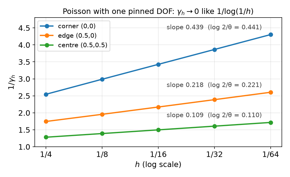
1/\gamma_h grows by a constant per halving of h, \approx\log2/\theta (\theta = interior angle at p: \pi/2, \pi, 2\pi). So \gamma_h\sim\theta/\log(1/h)\to0: no h-uniform stability.

2D: v can be pulled to 0 at a point at an energy cost \to0. The theorem needs |\Gamma_D|>0.
1D: H^1\subset C^0, one point is enough.
“Pin one DOF” for pure Neumann works only with compatible data (§C4).

§A9 Robin conditions

b(u,v)=\int_\Omega\nabla u\cdot\nabla v+\alpha\int_{\partial\Omega}uv, \alpha>0, on all of H^1:

Continuous: |b(u,v)|\le|u|_{H^1}|v|_{H^1}+\alpha\|u\|_{L^2(\partial\Omega)}\|v\|_{L^2(\partial\Omega)}\le(1+\alpha C_T^2)\|u\|_{H^1}\|v\|_{H^1} — trace inequality.
Coercive: b(v,v)=|v|^2_{H^1}+\alpha\|v\|^2_{L^2(\partial\Omega)} controls \|v\|^2_{L^2} by a Friedrichs-type inequality — HW6 Q1.

P1, N=32	\alpha=0.01	0.1	1	10	100	10^4
\gamma_h=\lambda_{\min}(K+\alpha B,\,G)	0.0399	0.3893	0.9405	0.9510	0.9518	0.9519

\alpha\to0: \gamma\approx\alpha|\partial\Omega|/|\Omega|=4\alpha (attained by constants) — Neumann.
\alpha\to\infty: \gamma\to2\pi^2/(1+2\pi^2)=0.9518 — the Dirichlet value of §A7.

§A10 Summary and exercises

Problem	Space	Coercivity from	F bounded by
Helmholtz, Neumann	H^1	b=(\cdot,\cdot)_{H^1}	Cauchy–Schwarz + trace (for g)
Poisson, pure Neumann	\int v=0	mean estimate; data must satisfy \int f+\int g=0	trace
Poisson, partial Dirichlet	v=0 on \Gamma_D, \|\Gamma_D\|>0	mean estimate + trace	trace
Poisson, Robin	H^1	trace + Friedrichs-type	trace

Exercise A.1 — Compatibility

For -\Delta u+cu=f, \partial_nu=g with a constant c>0, is a compatibility condition needed? Why not?

Exercise A.2 — One dimension

On (0,1) with v(0)=0 show |v(x)|\le\sqrt x\,\|v'\|_{L^2} and hence \|v\|_{L^2}\le\tfrac1{\sqrt2}|v|_{H^1}. Why does this argument fail in 2D for a single point?

Part B — Dirichlet Conditions in DOLFINx

§B1 Essential conditions in the linear system

Split the DOFs into free (I) and Dirichlet (D) ones, \mathbf u_D=\mathbf g: \begin{bmatrix}A_{II}&A_{ID}\\A_{DI}&A_{DD}\end{bmatrix}\begin{bmatrix}\mathbf u_I\\\mathbf u_D\end{bmatrix}=\begin{bmatrix}\mathbf b_I\\\mathbf b_D\end{bmatrix} \quad\longrightarrow\quad A_{II}\,\mathbf u_I=\mathbf b_I-A_{ID}\,\mathbf g . The rows of D are test functions that are not in V_D — they are dropped; the columns of D multiply known values and move to the right.

DOLFINx keeps the full size and solves the symmetric system \begin{bmatrix}A_{II}&0\\0&I\end{bmatrix}\begin{bmatrix}\mathbf u_I\\\mathbf u_D\end{bmatrix}=\begin{bmatrix}\mathbf b_I-A_{ID}\mathbf g\\\mathbf g\end{bmatrix}

Step	Function
zero rows and columns of D, put 1 on the diagonal	`assemble_matrix(a, bcs=[bc])`
\mathbf b_I\leftarrow\mathbf b_I-A_{ID}\mathbf g (“lifting”)	`apply_lifting(b, [a], bcs=[[bc]])`
\mathbf b_D\leftarrow\mathbf g	`set_bc(b, [bc])`

§B2 Finding the boundary DOFs

# by DOF coordinates (Lagrange elements: DOFs are point values)
dofs = fem.locate_dofs_geometrical(V, lambda x: np.isclose(x[0], 0.0))

# by mesh entities: all DOFs on the given facets (vertices, edge midpoints, ...)
fdim = msh.topology.dim - 1
msh.topology.create_connectivity(fdim, msh.topology.dim)
facets = mesh.locate_entities_boundary(msh, fdim, lambda x: np.isclose(x[0], 0.0))
dofs = fem.locate_dofs_topological(V, fdim, facets)          # or ft.find(tag) from facet tags

Left side of the 8\times8 unit square:

marker	P1	P2
`np.isclose(x[0], 0)`	9	17
topological, left facets	9	17
`x[0] == 0.0`	0	0
`x[0] == 1.0` (right side)	0	8

The DOF coordinates on x=0 are \pm2.7\times10^{-18}, not 0 (Week 4: x**a gave nan for the same reason). Exact float comparison finds nothing — no error, just a missing boundary condition.

§B3 `fem.dirichletbc` in 0.11

bc = fem.dirichletbc(0.0, dofs, V)                         # constant value: pass V
bc = fem.dirichletbc(fem.Constant(msh, 1.0), dofs, V)      # Constant: pass V

g = fem.Function(V)                                        # space-dependent value
g.interpolate(lambda x: np.sin(np.pi * x[1]))              # NumPy callable, or
g.interpolate(fem.Expression(u_ex, V.element.interpolation_points))   # a UFL expression (MMS)
bc = fem.dirichletbc(g, dofs)                              # Function: V is taken from g

Call	0.11
`dirichletbc(g, dofs)` with `g` a `Function`	✅
`dirichletbc(g, dofs, V)` with `g` a `Function`	`TypeError: __init__(): incompatible function arguments`
several boundary parts	one `bc` per part, `bcs=[bc_left, bc_right]`

For a sub-space (vector or mixed problems, Week 11) the DOFs come from locate_dofs_topological((V.sub(0), V0), ...) — geometrical location needs DOF coordinates, the topological one always works.

§B4 The assembly pipeline

a, L = fem.form(a_ufl), fem.form(L_ufl)
A = assemble_matrix(a, bcs=[bc]); A.assemble()                 # rows and columns of D zeroed, diagonal 1
b = assemble_vector(L)
apply_lifting(b, [a], bcs=[[bc]])                              # b_I -= A_ID g   (each rank, incl. ghosts)
b.ghostUpdate(addv=PETSc.InsertMode.ADD, mode=PETSc.ScatterMode.REVERSE)   # ghosts → owners
set_bc(b, [bc])                                                # b_D = g         (owned entries only)
ksp.solve(b, uh.x.petsc_vec); uh.x.scatter_forward()

LinearProblem(a_ufl, L_ufl, bcs=[bc], petsc_options_prefix=..., ...) performs exactly these steps.

The order matters. set_bc writes \mathbf g into owned entries. A later ghostUpdate(ADD) adds the other rank’s contributions on top of it — the Dirichlet values are corrupted, but only in DOFs that are also ghosts on another rank.

§B5 Pipeline mistakes, measured

Mixed problem of §C2 (Dirichlet + Neumann + Robin), P1, -np 2, L^2 error:

	N=8	16	32	64	symptom
correct	1.9e-2	4.9e-3	1.2e-3	3.1e-4	rate 2
no `apply_lifting`	0.55	0.57	0.59	0.60	stagnates
`assemble_matrix(a)` without `bcs`	15	26	47	90	grows
`set_bc` before `ghostUpdate`	1.9e-2	1.6e-2	1.2e-3	3.1e-4	one mesh only (here N=16; on Colab N=64), only with `-np 2`

Without lifting the free rows still “see” \mathbf u_D=0: the solution is that of g_D=0 in the interior, glued to g_D on \Gamma_D.
The ordering bug is invisible with -np 1, and which mesh it hits depends on the partition — only a rate table and a parallel run catch it.

Part C — Neumann, Robin, Subdomains

§C1 Boundary markers and `ds(i)`

LEFT, RIGHT, BOTTOM, TOP = 1, 2, 3, 4
facets, values = [], []
for tag, marker in ((LEFT,   lambda x: np.isclose(x[0], 0)), (RIGHT, lambda x: np.isclose(x[0], 1)),
                    (BOTTOM, lambda x: np.isclose(x[1], 0)), (TOP,   lambda x: np.isclose(x[1], 1))):
    f = mesh.locate_entities_boundary(msh, fdim, marker)
    facets.append(f); values.append(np.full(len(f), tag, dtype=np.int32))
facets, values = np.hstack(facets), np.hstack(values)
order = np.argsort(facets)                                   # meshtags expects sorted indices
ft = mesh.meshtags(msh, fdim, facets[order], values[order])

ds = ufl.Measure("ds", domain=msh, subdomain_data=ft)
L = f * v * ufl.dx + g_N * v * ds(TOP) + g_N * v * ds(BOTTOM) + r * v * ds(RIGHT)
bc = fem.dirichletbc(g_D, fem.locate_dofs_topological(V, fdim, ft.find(LEFT)))

Check the tags: \int 1\,ds(i) must be the length of side i. Without subdomain_data the same code runs, and \int1\,ds(1)=0 — every ds(i) term silently disappears (§D1).

§C2 MMS with all three conditions

\tilde u=1+\sin(\pi x)e^{y}+xy^2 — no special boundary behaviour needed: all boundary data are computed from \tilde u.

n = ufl.FacetNormal(msh)
f   = -ufl.div(ufl.grad(u_ex))
g_N = ufl.dot(ufl.grad(u_ex), n)                     # Neumann data on top and bottom (normal from UFL)
r   = ufl.dot(ufl.grad(u_ex), n) + alpha * u_ex      # Robin data on the right, alpha = 10
g_D = fem.Function(V); g_D.interpolate(fem.Expression(u_ex, V.element.interpolation_points))   # left
a = inner(grad(u), grad(v)) * dx + alpha * u * v * ds(RIGHT)

-np 2, LU:

	\\|e\\|_{L^2}, N=8\to64	rates	\|e\|_{H^1} rates
P1	1.94e-2 → 3.08e-4	1.98, 2.00, 2.00	0.99, 1.00, 1.00
P2	4.68e-4 → 9.36e-7	2.98, 2.99, 2.99	1.98, 1.99, 2.00

Week 5 had to pick \tilde u with \partial_n\tilde u=0 because g=0 was hard-wired. With boundary terms in F, any smooth \tilde u works.

§C3 Pure Neumann in PETSc

K is singular, K\mathbf 1=\mathbf 0. Tell the solver:

ns = PETSc.NullSpace().create(constant=True, comm=msh.comm)
A.setNullSpace(ns)                   # Krylov methods work orthogonal to the constant vector
ns.remove(b)                         # project b: sum_i b_i = 0
ksp.setType("cg"); ksp.getPC().setType("hypre")
ksp.solve(b, uh.x.petsc_vec); uh.x.scatter_forward()
mean = msh.comm.allreduce(fem.assemble_scalar(fem.form(uh * ufl.dx)), op=MPI.SUM)
uh.x.array[:] -= mean                # the nullspace fixes sum_i u_i, not the integral of u_h

Compatible data (\tilde u=\cos\pi x\cos\pi y+x^2y, f, g by UFL), -np 2: CG + hypre needs 7–8 iterations for every N; rates P1 1.95, 1.99, 2.00 and P2 2.98, 2.99, 3.00 (L^2). Without the last two lines, \int u_h is of order 10^{-3} instead of 0: harmless for gradients, wrong for a comparison with \tilde u.

§C4 Pure Neumann with incompatible data

f\to f+1, so \int f+\int g=1. P1, -np 2; error of u_h-\bar u_h against \tilde u-\bar{\tilde u}:

Strategy	KSP reason	\\|e\\|_{L^2}, N=8\to64	\max\|u_h\|
nullspace + `remove(b)`, CG	2	2.4e-2 → 9.4e-4, rates 1.79, 1.59, 1.31	1.8
nullspace, `b` not projected, CG	−8, −8, −8, −4	4.8e-2 → 5.7\times10^4	up to 2\times10^{11}
pin one DOF (corner), LU	4	0.26 → 0.25, stagnates	4.2 → 5.5, grows
plain LU	4	erratic	10^{12}–10^{14}

remove(b) subtracts the same number from every entry of \mathbf b — that is not the load vector of a constant (boundary DOFs carry less weight), so it solves a nearby problem.
Pinning turns the defect into a point source at the pinned corner: \max|u_h| grows by 0.44 per halving of h =\log2/(\pi/2), the \log(1/r) of §A8.
With compatible data all four strategies give the same errors. Print \int f+\int g before solving.

§C5 Subdomains and multi-material problems

-\nabla\cdot(k\nabla u)=f with k=k_1 in \Omega_1, k=k_2 in \Omega_2. Weak form unchanged: \int_\Omega k\nabla u\cdot\nabla v.

Interface conditions on \Gamma=\partial\Omega_1\cap\partial\Omega_2:

[u]=0 — built into V_h\subset H^1 (continuous elements)
[k\,\partial_nu]=0 (flux continuity) — natural: comes out of the integration by parts, nothing to impose

u has a kink on \Gamma: it is smooth on each side, but not in H^2(\Omega).

Q = fem.functionspace(msh, ("DG", 0)); k = fem.Function(Q)          # one value per cell
k.x.array[ct.find(1)] = 10.0; k.x.array[ct.find(2)] = 1.0           # from cell tags (Gmsh)
# or: cells = mesh.locate_entities(msh, tdim, lambda x: x[0] <= 0.5 + 1e-12)
a = k * ufl.inner(ufl.grad(u), ufl.grad(v)) * ufl.dx

dx = ufl.Measure("dx", domain=msh, subdomain_data=ct)               # alternative: one term per material
a = 10.0 * ufl.inner(ufl.grad(u), ufl.grad(v)) * dx(1) + 1.0 * ufl.inner(ufl.grad(u), ufl.grad(v)) * dx(2)

§C6 The mesh must follow the interface

Layered square, k=1 for x<s, k=10 for x>s; \tilde u=\cos(\pi y)\cdot\{\sin(\pi x)/k_i+c_i\} has continuous u and k\,\partial_xu. -np 2, LU:

interface	element	L^2 rates (N=8\to64)	H^1 rates
s=1/2 — on mesh lines	P1	1.98, 1.99, 2.00	1.00, 1.00, 1.00
	P2	3.01, 3.00, 3.00	1.99, 2.00, 2.00
s=1/3 — cuts through cells	P1	0.57, 1.84, 0.26	1.07, 0.47, 0.92
	P2	1.02, 0.94, 1.03	1.68, −0.65, 1.71

On a fitted mesh, u is smooth on every cell: the interpolation estimate of Week 4 applies cell by cell → full rates.
On a cut mesh, cells contain the kink: rate about 1 in L^2, erratic, and P2 is no better than P1. Fix the mesh, not the element.

§C7 Gmsh: geometry → tagged mesh

import gmsh
from dolfinx.io import gmsh as gmshio
gmsh.initialize()
if comm.rank == 0:                               # build the model on one rank
    outer = gmsh.model.occ.addDisk(0, 0, 0, 1, 1)
    inner = gmsh.model.occ.addDisk(0, 0, 0, 0.5, 0.5)
    gmsh.model.occ.fragment([(2, outer)], [(2, inner)])   # conforming interface
    gmsh.model.occ.synchronize()
    gmsh.model.addPhysicalGroup(2, [s_in], 1); gmsh.model.addPhysicalGroup(2, [s_out], 2)   # → cell tags
    gmsh.model.addPhysicalGroup(1, outer_curves, 10)                                        # → facet tag
    gmsh.option.setNumber("Mesh.CharacteristicLengthMax", 0.1)
    gmsh.model.mesh.generate(2)
md = gmshio.model_to_mesh(gmsh.model, comm, 0, gdim=2)   # every rank
gmsh.finalize()
msh, ct, ft = md.mesh, md.cell_tags, md.facet_tags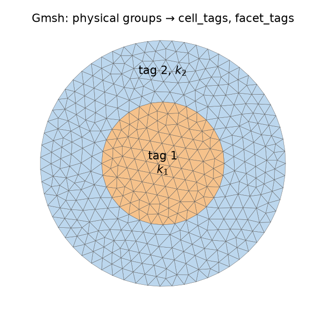

h=0.1: 817 cells (212 inclusion, 605 matrix), 63 outer facets (Gmsh 4.15; counts depend on the version).

Only entities in a physical group become part of the mesh; the group tags become cell_tags / facet_tags.

§C8 Gmsh disk: geometry limits the rate

k_1=10 for r<\tfrac12, k_2=1; u=0 on r=1; exact u=\cos(\pi r/2)/k_i+c_i. -np 2, L^2 error, Gmsh size h=0.2\to0.025:

mesh	element	L^2 rates
interface meshed (`fragment`)	P1	2.04, 1.99, 2.00
	P2, straight-sided triangles	2.01, 2.02, 2.01
	P2, curved triangles (`gmsh.model.mesh.setOrder(2)`)	3.28, 2.97, 3.02
interface not meshed (k from cell midpoints)	P1	1.46, 0.74, 1.28

Straight-sided cells replace the circles by polygons: an O(h^2) geometry error that P2 cannot beat. Curved (isoparametric) cells restore h^3.
A curved interface that the mesh ignores costs as much as the misaligned layer of §C6.

§C9 Math → DOLFINx

Math	DOLFINx 0.11
\Gamma_D,\Gamma_N,\Gamma_R	`mesh.meshtags(msh, fdim, facets_sorted, tags)`, or `md.facet_tags` from Gmsh
u=g_D on \Gamma_D	`fem.dirichletbc(g, fem.locate_dofs_topological(V, fdim, ft.find(i)))`
\int_{\Gamma_N}g_Nv, \alpha\int_{\Gamma_R}uv	`g * v * ds(i)`, `alpha * u * v * ds(j)` with `ds = Measure("ds", subdomain_data=ft)`
\partial_n\tilde u	`ufl.dot(ufl.grad(u_ex), ufl.FacetNormal(msh))`
lifting \mathbf b_I-A_{ID}\mathbf g	`assemble_matrix(a, bcs)`, `apply_lifting`, `ghostUpdate`, `set_bc` — in this order
\int v=0 (pure Neumann)	`PETSc.NullSpace().create(constant=True)`, `A.setNullSpace`, `ns.remove(b)`, subtract the mean
k per material	DG0 `Function` from `cell_tags`, or `dx(i)` with `subdomain_data=ct`
geometry	Gmsh physical groups → `dolfinx.io.gmsh.model_to_mesh`

Part D — LLMs and Boundary Conditions · Assignment

§D1 Where LLM-generated BC code goes wrong

Kind	What it looks like	Detection
Stale API	`dirichletbc(g_func, dofs, V)`; `LinearProblem` without prefix; `from dolfinx.io import gmshio`; `msh, ct, ft = model_to_mesh(...)`	`TypeError`, `ImportError`, `ValueError` at once
Silent location bugs	`x[0] == 0` — finds 0 DOFs on P1 and P2; the problem stays solvable	count DOFs, \int1\,ds(i)
Silent measure bugs	`ds(i)` without `subdomain_data` (integral = 0); `dx` instead of `ds`	\int1\,ds(i); rates
Wrong data	\partial_nu written as \partial_yu on the bottom side (\mathbf n=(0,-1)); Robin term only in L	error stagnates
Pipeline	no `apply_lifting`; `set_bc` before `ghostUpdate`; `assemble_matrix` without `bcs`	rates; `-np 1` vs `-np 2`
Pure Neumann	LU on the singular matrix; no compatibility check; mean not removed	reason, \max\|u_h\|, \int f+\int g

§D2 Verify each boundary separately

Checklist for a BC-heavy solver

Print the number of DOFs on each Dirichlet part and \int 1\,ds(i) for each tag.
MMS with every condition active, all data computed from \tilde u by UFL (normals from FacetNormal).
Rates over ≥ 3 meshes, P1 and P2.
Same numbers with -np 1 and -np 2.
Pure Neumann: \int f+\int g, KSP reason, \max|u_h|, mean removed.
Multi-material: look at the mesh — does it follow the interfaces?

A boundary condition that is missing usually leaves a solvable problem: wrong, but no error message. A rate table is the only alarm.

Assignment — HW6, due before the Week 7 lecture

HW6 — Multi-material and Robin conditions (100)

Q1 proofs: pure Neumann with boundary data, Robin coercivity, Dirichlet lifting in matrix form (25)
Q2 composite wall: two materials, Dirichlet + insulated + convective (Robin) sides, heat generation; exactness, rates, fitted vs cut interface (35)
Q3 coercivity constants: Robin, and one pinned DOF at a corner, an edge and an interior point (20)
Q4 LLM-generated mixed-BC solver with planted bugs: find, fix, explain (20)

Submit the executed .ipynb (restart & run all) with the AI-usage log.

Reminder: an error in a %%fenicsx cell does not stop Run all. Read every output before you submit.

Summary

Concept	Key idea	DOLFINx
Essential / natural	Dirichlet in the space; Neumann, Robin in the forms	`dirichletbc`; `ds(i)`
Poincaré-type inequality	\\|v\\|_{L^2}\le C\|v\|_{H^1} on the space ⇒ \gamma=1/(1+C^2)	\gamma_h=\lambda_{\min}
Pure Neumann	mean estimate; \int f+\int g=0; u up to a constant	`NullSpace`, `remove(b)`, subtract mean
Trace inequality	\\|u\\|_{L^2(\partial\Omega)}\le C\\|u\\|_{H^1}; lines yes, points no	`ds` data bounded
Partial Dirichlet	needs \|\Gamma_D\|>0; one pinned DOF: \gamma_h\sim1/\log(1/h)	`locate_dofs_topological`
Lifting	A_{II}\mathbf u_I=\mathbf b_I-A_{ID}\mathbf g	`apply_lifting` → `ghostUpdate` → `set_bc`
Multi-material	flux continuity is natural; the mesh must follow the interface	DG0 k, `cell_tags`, Gmsh

Next week — Convergence theory

Sobolev spaces, Céa’s lemma, elliptic regularity, Aubin–Nitsche: why the rates are k and k+1 — and when they are not.