AI-based Materials and Process Simulation II
Week 04 — J2 Plasticity: Return Mapping, Quadrature Spaces, the Consistent Tangent, Limit Loads
Process Systems Laboratory
Department of Chemical and Biomolecular Engineering, SeoulTech
Today
| Part | Topic | Time |
|---|---|---|
| Quiz on Week 3 (closed-AI) | 10 min | |
| A | Theory — J2 plasticity, backward Euler, radial return, the consistent tangent, the thick tube (first yield, limit load) | 55 min |
| B | Plasticity in code — quadrature spaces, the update in NumPy, an explicit Newton loop, displacement control | 45 min |
| C | Verification — material-point tests, elastic and first-yield checks, Newton rates, limit load, a 1D reference | 40 min |
| D | LLM pitfalls · assignment | 20 min |
Lab notebook: W04_lab.ipynb · Assignment: W04_HW4.ipynb (due before Week 5)
Week 3 in one slide
- One 3D law, three 2D reductions by the choice of \varepsilon_{zz}; GPS adds one number e_0, eliminated by static condensation (two solves, one LU).
- Thermal stress -\beta\Delta T\,\mathbf I; harmonic \Delta T is stress-free with statically determinate supports; full coupling slows heat by 1+\delta.
- Verification by exact answers that are not zero for the thing being tested.
Today: the first path-dependent material. The stress is no longer a function of the strain — it is the result of an update that remembers the past. New in code: data at quadrature points and a Newton loop we write ourselves.
Part A · J2 plasticity
Small-strain plasticity: the equations
\boldsymbol\varepsilon=\boldsymbol\varepsilon^e+\boldsymbol\varepsilon^p,\qquad \boldsymbol\sigma=\mathbb C:(\boldsymbol\varepsilon-\boldsymbol\varepsilon^p),\qquad f(\boldsymbol\sigma,p)=\sigma_{\rm eq}-(\sigma_0+Hp)\le0,\qquad \sigma_{\rm eq}=\sqrt{\tfrac32\,\mathbf s:\mathbf s}
| Ingredient | J2 (von Mises) with linear isotropic hardening |
|---|---|
| deviator | \mathbf s=\boldsymbol\sigma-\tfrac13(\operatorname{tr}\boldsymbol\sigma)\mathbf I — all three normal components, also in a 2D model |
| flow rule (normality) | \dot{\boldsymbol\varepsilon}^p=\dot p\,\dfrac{\partial f}{\partial\boldsymbol\sigma}=\dot p\,\dfrac32\,\dfrac{\mathbf s}{\sigma_{\rm eq}} — deviatoric: plastic flow keeps the volume |
| equivalent plastic strain | \dot p=\sqrt{\tfrac23\,\dot{\boldsymbol\varepsilon}^p:\dot{\boldsymbol\varepsilon}^p} (in uniaxial tension p=\varepsilon^p_{xx}) |
| loading/unloading | \dot p\ge0,\quad f\le0,\quad \dot p\,f=0 (Kuhn–Tucker) |
Two material constants beyond elasticity: \sigma_0 and H (H=0: perfect plasticity). Uniaxial tangent after yield: E_t=EH/(E+H).
Backward Euler: the return mapping
Step n\to n+1, strain increment \Delta\boldsymbol\varepsilon given (by the Newton iterate). With \mu the shear modulus:
- Elastic predictor: \boldsymbol\sigma^{\rm tr}=\boldsymbol\sigma_n+\mathbb C:\Delta\boldsymbol\varepsilon, \;f^{\rm tr}=\sigma_{\rm eq}^{\rm tr}-(\sigma_0+Hp_n). If f^{\rm tr}\le0: done, \boldsymbol\sigma=\boldsymbol\sigma^{\rm tr}.
- Plastic corrector: \boldsymbol\sigma=\boldsymbol\sigma^{\rm tr}-2\mu\,\Delta p\,\tfrac32\,\mathbf s/\sigma_{\rm eq}. The deviator shrinks along its own direction: \mathbf s=\big(1-3\mu\Delta p/\sigma^{\rm tr}_{\rm eq}\big)\mathbf s^{\rm tr}, so \sigma_{\rm eq}=\sigma^{\rm tr}_{\rm eq}-3\mu\Delta p, and f=0 gives
\Delta p=\frac{f^{\rm tr}}{3\mu+H},\qquad \boldsymbol\sigma=\boldsymbol\sigma^{\rm tr}-2\mu\sqrt{\tfrac32}\,\Delta p\,\hat{\mathbf n},\qquad \hat{\mathbf n}=\frac{\mathbf s^{\rm tr}}{\lvert\mathbf s^{\rm tr}\rvert},\quad \lvert\mathbf s\rvert=\sqrt{\tfrac23}\,\sigma_{\rm eq}
- Closed form for J2 + linear hardening — no local iteration. Exact on the discrete level: after the return f=0 to round-off.
- The return is radial in the deviatoric plane. The pressure \tfrac13\operatorname{tr}\boldsymbol\sigma is untouched.
The return in one picture
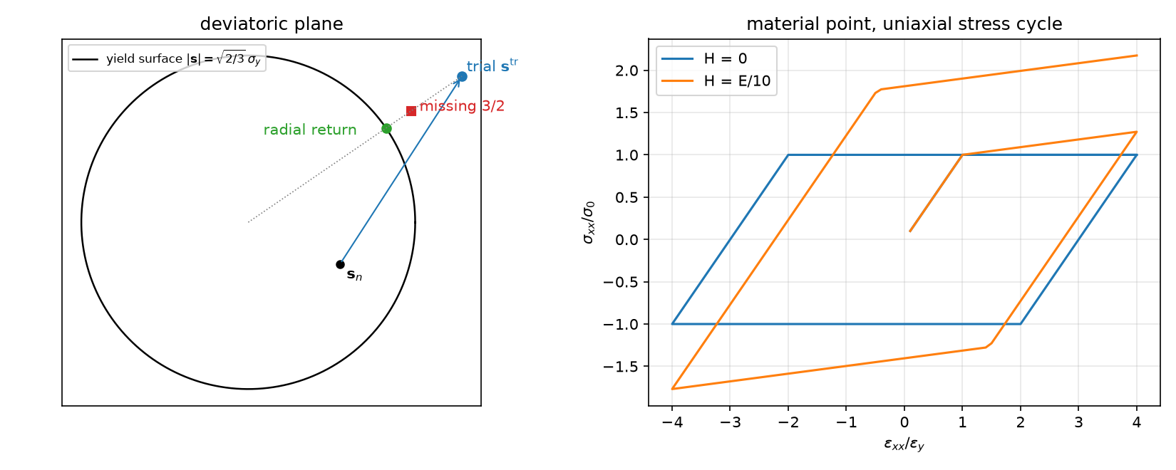
Left: the trial deviator outside the circle goes back to it along the radius. Right: one material point, uniaxial stress, strain-controlled cycle ±4 \varepsilon_y: with H=0 the stress stays at \pm\sigma_0; H=E/10 peaks at 318.18 MPa, the exact \sigma_0+E_t(4\varepsilon_y-\varepsilon_y).
The consistent tangent
Newton needs \partial\boldsymbol\sigma_{n+1}/\partial\Delta\boldsymbol\varepsilon of the discrete update, not of the rate equations:
\mathbb C^{\rm alg}=\mathbb C-2\mu\,\beta\,\mathbb I_{\rm dev}-2\mu\,\bar\theta\,\hat{\mathbf n}\otimes\hat{\mathbf n},\qquad \beta=\frac{3\mu\,\Delta p}{\sigma^{\rm tr}_{\rm eq}},\qquad \bar\theta=\frac{3\mu}{3\mu+H}-\beta
- Elastic points: \Delta p=0 → \mathbb C^{\rm alg}=\mathbb C. Symmetric (associative flow).
- \beta\,\mathbb I_{\rm dev}: the deviator is scaled down; \bar\theta\,\hat{\mathbf n}\otimes\hat{\mathbf n}: no stiffness along the flow direction (for H=0).
- With \mathbb C^{\rm alg} Newton converges quadratically; with the elastic \mathbb C (“modified Newton”) linearly, and the rate degrades as the plastic zone grows.
- Check in code: compare \mathbb C^{\rm alg} with a finite difference of
update— relative difference 3\times10^{-11} (the elastic \mathbb C: 0.25).
Mandel notation for plane strain
Store symmetric tensors as 4-vectors so that \boldsymbol\sigma:\boldsymbol\varepsilon is a dot product:
\boldsymbol\sigma\mapsto(\sigma_{xx},\sigma_{yy},\sigma_{zz},\sqrt2\,\sigma_{xy}),\qquad \boldsymbol\varepsilon\mapsto(\varepsilon_{xx},\varepsilon_{yy},\varepsilon_{zz},\sqrt2\,\varepsilon_{xy}),\qquad \mathbb C=\lambda\,\mathbf m\mathbf m^\top+2\mu\,\mathbf I_4,\quad \mathbf m=(1,1,1,0)
- Plane strain: \varepsilon_{zz}=0, but \sigma_{zz}\ne0 and it enters \mathbf s and \sigma_{\rm eq}. The 4th component is not optional.
- \mathbb I_{\rm dev}=\mathbf I_4-\tfrac13\mathbf m\mathbf m^\top, \;\lvert\mathbf s\rvert^2=\mathbf s\cdot\mathbf s (the \sqrt2 makes the shear count twice).
- The same 4-vector works for the 1D radial model of a tube: (\varepsilon_{rr},\varepsilon_{\theta\theta},\varepsilon_{zz},0)=(u',u/r,0,0).
The thick tube: elastic state and first yield
Plane strain, inner radius a, outer b, inner pressure p. Lamé: \sigma_{rr}=A-B/r^2, \sigma_{\theta\theta}=A+B/r^2, \sigma_{zz}=2\nu A, with A=pa^2/(b^2-a^2), B=Ab^2. At r=a:
\sigma_{\rm eq}^2=\frac{3B^2}{a^4}+(1-2\nu)^2A^2\quad\Rightarrow\quad p_y=\frac{\sigma_0\,(b^2-a^2)}{\sqrt{3b^4+(1-2\nu)^2a^4}}
- \nu=\tfrac12: p_y=\frac{\sigma_0}{\sqrt3}\big(1-\frac{a^2}{b^2}\big) — the textbook formula; it assumes \sigma_{zz} = the mean of \sigma_{rr},\sigma_{\theta\theta}.
- Our tube (a=1, b=1.3, E=70 GPa, \nu=0.3, \sigma_0=250 MPa): p_y=58.39 MPa; the \nu=\tfrac12 formula gives 58.93 (+0.93 %).
The limit load
At collapse the stresses stop changing, so the strain rate is purely plastic. Plane strain: \dot\varepsilon_{zz}=\dot\varepsilon^p_{zz}=0 ⇒ s_{zz}=0 ⇒ \sigma_{zz}=\tfrac12(\sigma_{rr}+\sigma_{\theta\theta}) ⇒ \sigma_{\rm eq}=\tfrac{\sqrt3}{2}(\sigma_{\theta\theta}-\sigma_{rr})=\sigma_0. Equilibrium \partial_r\sigma_{rr}=(\sigma_{\theta\theta}-\sigma_{rr})/r from \sigma_{rr}(a)=-p to \sigma_{rr}(b)=0:
p_{\rm lim}=\frac{2\sigma_0}{\sqrt3}\ln\frac ba=75.74\ \text{MPa}\qquad\text{— no }E,\ \text{no }\nu
- Above p_{\rm lim} there is no equilibrium; at p_{\rm lim} the displacement is unbounded (perfect plasticity).
- Elastic–plastic boundary c (Hill, incompressible elastic zone, \nu=\tfrac12): \;p=\frac{\sigma_0}{\sqrt3}\big[2\ln\frac ca+1-\frac{c^2}{b^2}\big].
Part B · Plasticity in code
Where the variables live: quadrature spaces
\boldsymbol\sigma, p and \mathbb C^{\rm alg} are not finite element fields — they are values at the quadrature points, updated pointwise.
cell = msh.basix_cell()
Q4  = fem.functionspace(msh, basix.ufl.quadrature_element(cell, value_shape=(4,),   degree=2))   # sigma, d eps
Q44 = fem.functionspace(msh, basix.ufl.quadrature_element(cell, value_shape=(4, 4), degree=2))   # C_alg
Q1  = fem.functionspace(msh, basix.ufl.quadrature_element(cell, value_shape=(),     degree=2))   # p
sig, sig_n, Ct = fem.Function(Q4), fem.Function(Q4), fem.Function(Q44)
p, p_n = fem.Function(Q1), fem.Function(Q1)- Degree 2 on triangles = 3 points per cell;
sig.x.array.reshape(-1, 4)is a plain (n_q,4) NumPy array. - A form with a quadrature function is integrated at those points — FFCx takes the rule from the element (measured: the
quadrature_degreemetadata is ignored). - Two copies: the converged state (\boldsymbol\sigma_n,p_n) and the current iterate (\boldsymbol\sigma,p).
Strain at the points, update in NumPy
def eps4(u):                                  # Mandel, plane strain
    e = ufl.sym(ufl.grad(u))
    return ufl.as_vector([e[0, 0], e[1, 1], 0, np.sqrt(2) * e[0, 1]])

deps_expr = fem.Expression(eps4(Du), Q4.element.interpolation_points)   # compiled once
deps = fem.Function(Q4)

def constitutive():
    deps.interpolate(deps_expr)                                         # evaluate at all quadrature points
    s, pp, C, pl = mat.update(deps.x.array.reshape(-1, 4), sig_n.x.array.reshape(-1, 4), p_n.x.array)
sig.x.array[:] = s.ravel(); p.x.array[:] = pp; Ct.x.array[:] = C.ravel()Duis the displacement increment since the last converged step;updateis vectorised over all points (j2.py, NumPy only).- The material law knows nothing about DOLFINx: you can test it in an ordinary notebook cell.
Residual and Jacobian
R(\mathbf v)=\int_\Omega\boldsymbol\sigma\cdot\boldsymbol\varepsilon(\mathbf v)\,dA-\int_{\Gamma_i}(-p\,\mathbf n)\cdot\mathbf v\,ds,\qquad J(\delta\mathbf u,\mathbf v)=\int_\Omega\big(\mathbb C^{\rm alg}\boldsymbol\varepsilon(\delta\mathbf u)\big)\cdot\boldsymbol\varepsilon(\mathbf v)\,dA
sigandCtare coefficients, not UFL expressions ofu: UFL cannot differentiate through the return mapping, so we supply the tangent.- 1D radial model: the same forms with (u',u/r,0,0) and the weight r (
* x[0] * dx).
The Newton loop
def step(load):
    Du.x.array[:] = 0.0;  pload.value = load
    for it in range(maxit + 1):
        constitutive()                                  # sigma, p, C_alg from Du
        res = residual()                                # assemble F, lifting, set_bc
        if it == 0: ref = max(ref, res)
        if res <= rtol * ref: break                     # converged
        if it == maxit: return False                    # NOT converged: do not commit
        A.zeroEntries(); assemble_matrix(A, J, bcs=bcs); A.assemble()
        ksp.solve(b, du.x.petsc_vec); du.x.scatter_forward()
        Du.x.array[:] -= du.x.array
    u.x.array[:] += Du.x.array                          # commit: the new converged state
    sig_n.x.array[:] = sig.x.array;  p_n.x.array[:] = p.x.array
return True- The state is committed once per step, after convergence. Iterates never touch (\boldsymbol\sigma_n,p_n).
ref= the largest first residual seen so far: a small last increment near p_{\rm lim} must not tighten the tolerance below round-off.- The function returns whether it converged. A non-converged step is not an exception — the caller must look.
Displacement control and the reaction
Prescribe the inner radial displacement instead of p. The increment enters through the first correction, by lifting with the converged tangent:
- Setting the boundary DOFs of
Duto the new value before the first solve puts the whole jump into one layer of cells: measured, the 2D tube’s first step (0.5\,u_y) did not converge in 50 iterations. - The pressure from the consistent reaction: p=\dfrac{1}{a\,\pi/2}\displaystyle\int_\Omega\boldsymbol\sigma\cdot\boldsymbol\varepsilon(\mathbf w_R)\,dA with any \mathbf w_R that equals \mathbf e_r on r=a and is admissible (here \mathbf e_r\,(b-r)/(b-a)) — Week 1’s reaction, one form.
The model modules
j2.py (NumPy) |
plas.py (DOLFINx) |
|---|---|
J2(E, nu, sig0, H): \mathbb C, update(deps, sig_n, p_n, tangent) |
annulus_mesh (curved, as Week 3), radial_mesh (1D) |
dev, von_mises, IDEV, ONE |
Tube(msh, ft, mat, ri, ro, control=, tangent=) |
uniaxial(mat, exx): one point in uniaxial stress |
step(load) → (converged, iterations, residuals) |
ur_inner, pressure_from_reaction, plastic_radius, max_von_mises |
|
lame_ur, p_first_yield, p_limit |
The same Tube runs the 2D quarter section and the 1D radial model. The 1D model with 400–800 cells is the reference for the 2D one — a different discretisation of the same problem, not a different program.
Part C · Verification
Material-point checks (no DOLFINx)
10^4 random strain increments from \boldsymbol\sigma_n=0, \lvert\Delta\varepsilon_{ij}\rvert\sim4\times10^{-3} (8244 points yield):
| Check | H=0 | H=E/10 |
|---|---|---|
| \max\lvert f\rvert/\sigma_0 at plastic points after the return | 1.1\times10^{-15} | 1.4\times10^{-15} |
| \max f/\sigma_0 at elastic points | <0 | <0 |
| \mathbb C^{\rm alg} vs central difference (h=10^{-8}) | 3.2\times10^{-11} | |
| elastic \mathbb C vs central difference | 0.25 | |
| uniaxial cycle: peak at 4\varepsilon_y vs \sigma_0+E_t\cdot3\varepsilon_y | 250 = 250 | 318.18 = 318.18 |
The local Newton of the uniaxial driver converges in one iteration: for linear hardening the update is piecewise linear and \mathbb C^{\rm alg} is exact.
Elastic and first-yield checks on the tube
- Elastic (p=0.5\,p_y, 2D, 8\times24 curved cells, P2): u_r(a)=1.6422404\times10^{-3} vs Lamé 1.6422406\times10^{-3} (relative 8\times10^{-8}), one Newton iteration.
- First yield (1D, 400 cells):
| load | plastic quadrature points |
|---|---|
| 0.999\,p_y(\nu=0.3) | 0 |
| 1.001\,p_y(\nu=0.3) | 1 |
| 0.999\times58.93 (the \nu=\tfrac12 formula) | 11 (zone up to c=1.0039) |
The textbook formula is not “approximately right” here — the model shows it is the formula of a different material.
Load–displacement and Newton
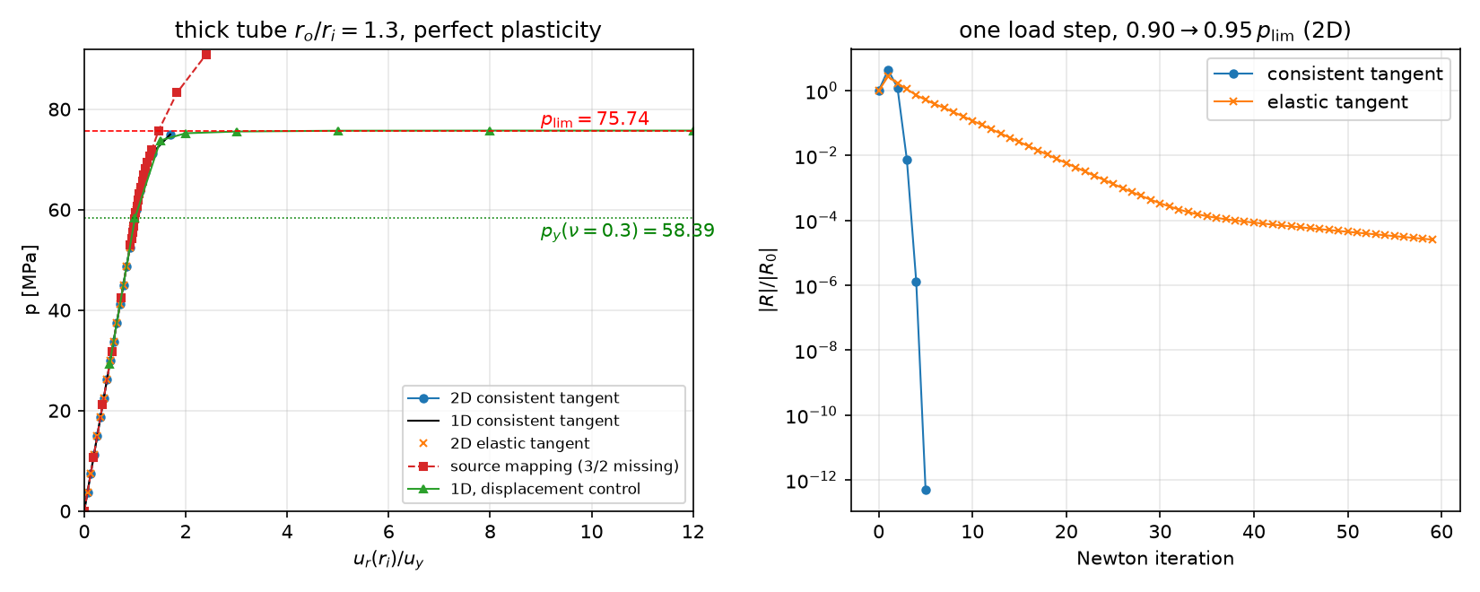
Left: 2D and 1D curves coincide; displacement control (green) follows the plateau at p_{\rm lim}. Right: one load step 0.90\to0.95\,p_{\rm lim} — consistent tangent 1,\,4.3,\,1.2,\,6.8\times10^{-3},\,1.4\times10^{-6},\,5\times10^{-13} (quadratic); elastic tangent a factor 0.74 per iteration (238 iterations to 10^{-8}).
Iterations per load step
20 equal steps of p from 0 to 0.99\,p_{\rm lim}, rtol = 10^{-8} (steps 1–15 elastic: one iteration each):
| step 16 | 17 | 18 | 19 | 20 (0.99\,p_{\rm lim}) | |
|---|---|---|---|---|---|
| 2D, consistent | 3 | 4 | 5 | 5 | 7 |
| 2D, elastic tangent | 49 | 86 | 124 | not converged (200) | |
| 1D, consistent | 4 | 4 | 5 | 5 | 8 |
| 1D, elastic tangent | 16 | 23 | 33 | 55 | not converged (200) |
- The elastic tangent is not “a bit slower”: its rate tends to 1 as the plastic zone spreads; near p_{\rm lim} it stalls.
- The consistent tangent costs nothing extra —
updatereturns it with the stress.
Mesh convergence and the 1D reference
u_r(a) at p=71.95 MPa (0.95\,p_{\rm lim}), load steps as in the original source, rtol 10^{-8}:
| model | u_r(a) [mm] |
|---|---|
| 2D 4\times12 / 8\times24 / 16\times48 | 4.51853 / 4.52049 / 4.51909 |
| 1D 50 / 200 / 800 | 4.51935 / 4.51930 / 4.51930 |
- 2D agrees with the 1D reference to 0.03 % on every mesh. The convergence is not monotone: the plastic front crosses quadrature points.
- Plastic radius at this load: 1D (800) 1.1711, 2D 16\times48 1.1656 (the radius of the outermost plastic quadrature point: resolution \sim h).
The limit load: pressure vs displacement control
| Pressure control (1D) | u_r(a)/u_y | converged |
|---|---|---|
| 75.0 / 75.5 / 75.7 / 75.73 MPa | 1.72 / 2.80 / 4.92 / 6.59 | yes (6–7 iterations) |
| 1.001\,p_{\rm lim}=75.81 MPa | — | no: 50 iterations, residual 10^2–10^3, not decreasing |
| Displacement control, u_r(a)=50\,u_y | p from the reaction [MPa] |
|---|---|
| 1D 400 | 75.73799 |
| 2D 4\times12 / 8\times24 / 16\times48 | 75.7388 / 75.7381 / 75.73804 |
| exact p_{\rm lim} | 75.73804 |
Exact: 75.738039. Coarse 2D meshes come out above it (a displacement model is too stiff: +10^{-5} on 4\times12); 16\times48 agrees to 7 digits. The 1D curve at 50\,u_y is still 5\times10^{-5} MPa below the asymptote.
The plastic zone
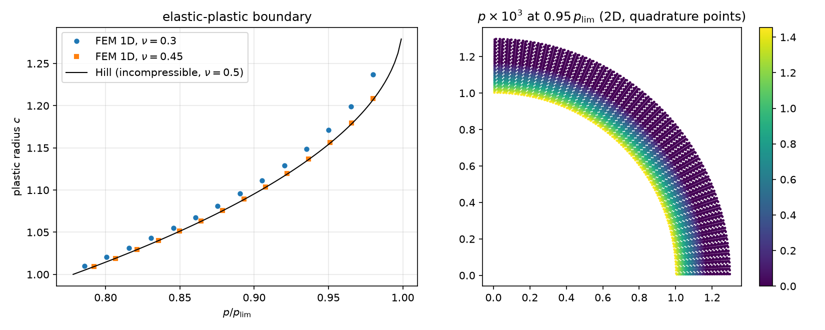
At 0.98\,p_{\rm lim}: c=1.2372 (\nu=0.3), 1.2087 (\nu=0.45), Hill 1.2070. Hill’s formula is exact only for an incompressible elastic zone: the model converges to it as \nu\to\tfrac12. Right: p is largest at the bore and zero outside c.
The original source, re-run on 0.11
The source of this week ran the same tube with its own return mapping: n = s/sigma_eq, sigma = sigma_tr - 2*mu*dgamma*n.
- \mathbf s/\sigma_{\rm eq} has length \sqrt{2/3}, not 1 — the factor \tfrac32 of the flow rule is missing. After the return f=f^{\rm tr}/3 (measured: ratio 0.3333); the stress stays outside the yield surface.
- Its tube: u_r(a)=4.3786 mm at 0.95\,p_{\rm lim} (0.11 reproduces the source’s printout to every digit) — 3.1 % stiff against 4.5193.
- The same mapping in our code converges at 1.2\,p_{\rm lim} with \sigma_{\rm eq}=1.27\,\sigma_0: a “perfectly plastic” model that hardens.
- Also in the source: the elastic tangent (11–15 iterations at a loose
1e-4), the \nu=\tfrac12 first-yield formula, the claim “FEM vs analytic ✅”.
Nothing crashed, the curve looked smooth and the iterations converged. One line — f\le0 after the return — would have caught it.
Part D · LLM pitfalls · assignment
What goes wrong in plasticity codes
| Pitfall | Measured symptom (this week) |
|---|---|
| Return with \mathbf s/\sigma_{\rm eq} instead of a unit normal (factor \tfrac32 lost) | f=f^{\rm tr}/3>0 after the return; tube 3.1 % stiff; converges above p_{\rm lim} |
| Elastic stiffness used as the Newton tangent | 49 → 124 iterations per step, no convergence at 0.99\,p_{\rm lim} (consistent: 3–7) |
| First-yield formula of \nu=\tfrac12 used for \nu=0.3 | 11 plastic points at “0.999 p_y”; the true p_y is 0.93 % lower |
| Pressure control beyond the limit load | no equilibrium: the step does not converge — silently, unless the code returns a flag |
| Prescribed displacement put into the boundary DOFs before the first solve | first 2D step diverges (50 iterations); lifting with the converged tangent: 1 iteration |
The fix is the same each time: a test whose exact answer you know before you run — f=0, a finite difference, Lamé, p_y, p_{\rm lim}.
Prompting for a plasticity model
- Paste the material update (
j2.py) and ask for material-point tests first: f\le0 after the return, a finite-difference tangent, a uniaxial curve. - State the kinematics: plane strain with \varepsilon_{zz}=0 and \sigma_{zz} kept; or the 1D radial model.
- Ask for an explicit Newton loop that returns convergence and commits the state only after convergence; say which tangent.
- State the load path, including where it must stop (p<p_{\rm lim}) or switch to displacement control.
- Ask for the analytical checks with the code: Lamé, p_y(\nu), p_{\rm lim}, a 1D reference.
Assignment HW4 (due before Week 5)
| Q | Topic | Points |
|---|---|---|
| 1 | Radial return, the consistent tangent, first yield and limit load of the tube (theory) | 20 |
| 2 | Hardening: the material point against the bilinear curve, the tube beyond p_{\rm lim}, Newton rates | 25 |
| 3 | Autofrettage: overload, unload, residual stress, reverse yielding in a thick tube (b/a=3) | 35 |
| 4 | Debugging an LLM-generated plasticity script | 20 |
Week 5 starts with a 10-minute quiz on today’s material (closed-AI).
Summary
| Concept | Key point | DOLFINx 0.11 |
|---|---|---|
| J2 plasticity | f=\sigma_{\rm eq}-(\sigma_0+Hp)\le0, deviatoric flow, \sigma_{zz} in the deviator | NumPy update on (n_q,4) arrays |
| Return mapping | \Delta p=f^{\rm tr}/(3\mu+H), radial; f=0 after the return | j2.py, testable without DOLFINx |
| Internal variables | values at quadrature points; converged copy + iterate | basix.ufl.quadrature_element, fem.Expression |
| Newton | consistent tangent → quadratic; commit after convergence | assemble_matrix(A, J, bcs), own loop |
| Limit load | no equilibrium above p_{\rm lim}; displacement control + reaction | apply_lifting(..., x0=[Du], alpha=-1) |
| Verification | material point, Lamé, p_y(\nu), p_{\rm lim}, 1D reference | Tube in 1D and 2D |
Next week: viscoelasticity and phase-field fracture — more internal variables, time-dependent and history fields.
