Process Dynamics and Control

6. Multi-loop Systems

Kee-Youn Yoo

Department of Chemical & Biomolecular Engineering, SeoulTech

What are we up to?

Single-loop feedback (Ch 4–5) reacts only after the controlled variable has moved. This chapter adds structure around the loop.

Strategy What it handles Key idea
Cascade (6.1) disturbances in the manipulated variable a fast inner loop fixes them before they reach the process
Feedforward (6.2–6.3) measured disturbances act on the disturbance itself, with a model
Ratio (6.4) streams that must stay in proportion one flow follows another
Smith predictor (6.5) large dead time feed back a prediction of the output
MIMO, RGA, decoupling (6.6–6.7) several interacting loops choose the pairing, then cancel the interaction

6.1 Cascade Control

The fired-heater problem

furnace cold process stream hot process stream T TT TC Ts​ fuel gas FT FC TC output = FC set point slave loop

The temperature controller (TC) does not move the valve directly: its output is the set point of a flow controller (FC), which holds the fuel-gas flow against upstream pressure changes.

Master and slave loops

  • Master (primary) controller TC: compares \(T\) with \(T^s\) and asks for a fuel-gas flow.
  • Slave (secondary) loop FC + FT + valve: delivers that flow, correcting supply-pressure upsets before they change the temperature.

To be effective, the slave loop must be much faster (smaller time constant) than the outer loop.

Design rules

  1. Tune the slave loop first, with the master in manual. Use as high a gain as feasible; P-only is usually enough.
  2. Then tune the master loop on the closed slave loop. Integral action belongs here, because it removes the offset.

Block diagram

R + − Gc​ + − Gc2​ Gv​ + + GL​ Gp​ L upstream fuel-gas pressure E p e2​ a C inner (slave) loop: fuel-gas flow outer (master) loop: temperature

\[ e_2=p-a,\qquad a=G_{c2}G_v\,e_2+G_LL \]

\[ a=\underbrace{\frac{G_{c2}G_v}{1+G_{c2}G_v}}_{G_v^*}\,p+\underbrace{\frac{G_L}{1+G_{c2}G_v}}_{G_L^*}\,L \]

Reduced block diagram

R + − Gc​ Gv​*​ + + GL​*​ Gp​ L C slave loop collapsed into Gv​*​, GL​*​

\[ C=\frac{G_cG_v^*G_p}{1+G_cG_v^*G_p}\,R+\frac{G_L^*G_p}{1+G_cG_v^*G_p}\,L \]

The slave loop turns the valve \(G_v\) into a faster, more accurate actuator \(G_v^*\), and it shrinks the load path to \(G_L^*\).

Example 6.1   Choosing the slave gain \(K_{c2}\)

PI master, P slave: \(\;G_p=\dfrac{0.8}{2s+1},\quad G_v=\dfrac{0.5}{s+1},\quad G_L=\dfrac{0.75}{s+1}\)

\[ G_v^*=\frac{K_{c2}K_v}{\tau_vs+1+K_{c2}K_v}=\frac{K_v^*}{\tau_v^*s+1} \] \[ \tau_v^*=\frac{\tau_v}{1+K_{c2}K_v},\qquad K_v^*=\frac{K_{c2}K_v}{1+K_{c2}K_v} \] \[ K_L^*=\frac{K_L}{1+K_{c2}K_v} \]

As \(K_{c2}\) grows: \(K_v^*\to1\) (the valve does what it is told), \(K_L^*\to0\) (load rejected), \(\tau_v^*\to0\) (faster).

\(K_{c2}\) \(\tau_v^*\) \(K_v^*\) \(K_L^*\)
0 1 — 0.75
2 0.50 0.50 0.375
5 0.29 0.71 0.21
18 0.10 0.90 0.075
50 0.04 0.96 0.029

(b) For \(\tau_v^*=0.1\tau_v\): \(\;1+0.5K_{c2}=10\Rightarrow K_{c2}=18\), giving \(K_v^*=0.9\) (10 % offset in the slave loop).

(c) Why P-only in the slave? The master PI removes the steady-state error in \(C\); the slave offset is harmless.

Example 6.1 (d): choosing the master \(\tau_I\)
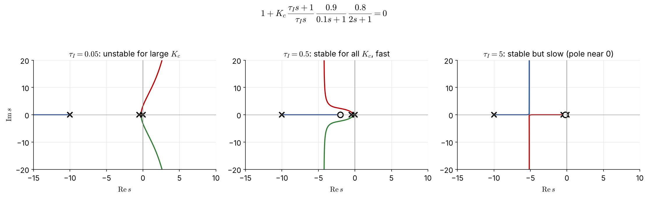
Poles \(0,\,-0.5,\,-10\); PI zero at \(-1/\tau_I\); \(\ n-m=2\), \(\ \gamma=\dfrac{-10.5+1/\tau_I}{2}\)

  • \(\tau_I=0.05\): \(\gamma=+4.75\) → unstable for \(K_c>1.54\)
  • \(\tau_I=0.5\): \(\gamma=-4.25\), stable for all \(K_c\), dominant poles far left
  • \(\tau_I=5\): stable, but a closed-loop pole is trapped near the zero at \(-0.2\) → slow

Choose \(\tau_I=0.5\): never unstable, and the fastest response.

Example 6.1 (e): without the cascade

\(\tau_I=0.5\), single loop:

\[ 1+K_c\,\frac{0.5s+1}{0.5s}\,\frac{0.5}{s+1}\,\frac{0.8}{2s+1}=0 \;\Rightarrow\; s^3+1.5s^2+(0.5+0.2K_c)s+0.4K_c=0 \]

Routh: \(\;1.5\,(0.5+0.2K_c)>0.4K_c\;\Rightarrow\;\) \(0<K_c<7.5\)

With the cascade the same master loop is stable for every \(K_c>0\). The slave loop removed the slow valve pole at \(-1\) and replaced it with a fast one at \(-10\).

Example 6.1: responses (replaces the Simulink runs)
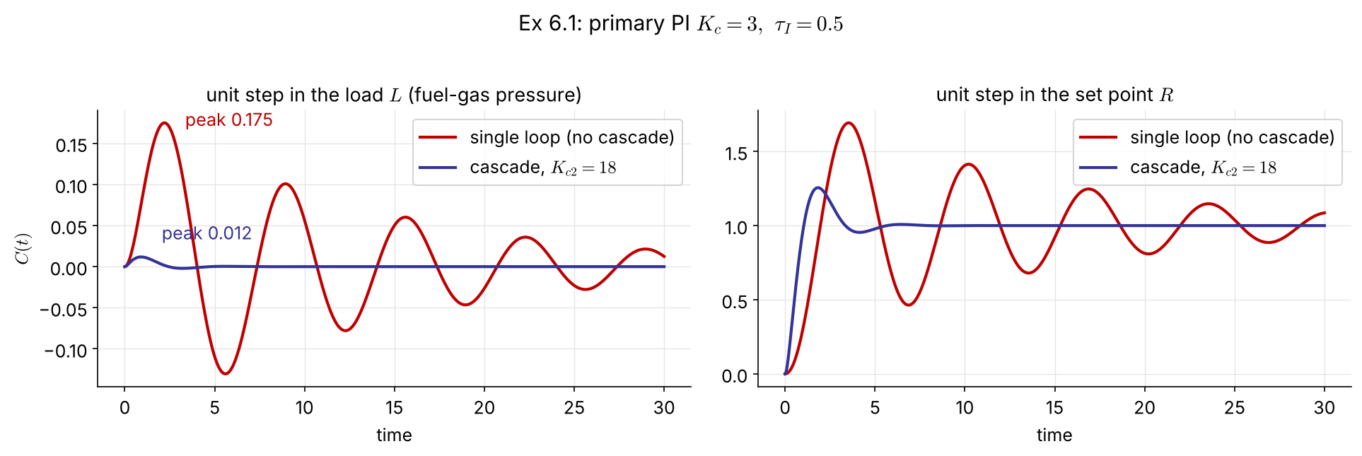
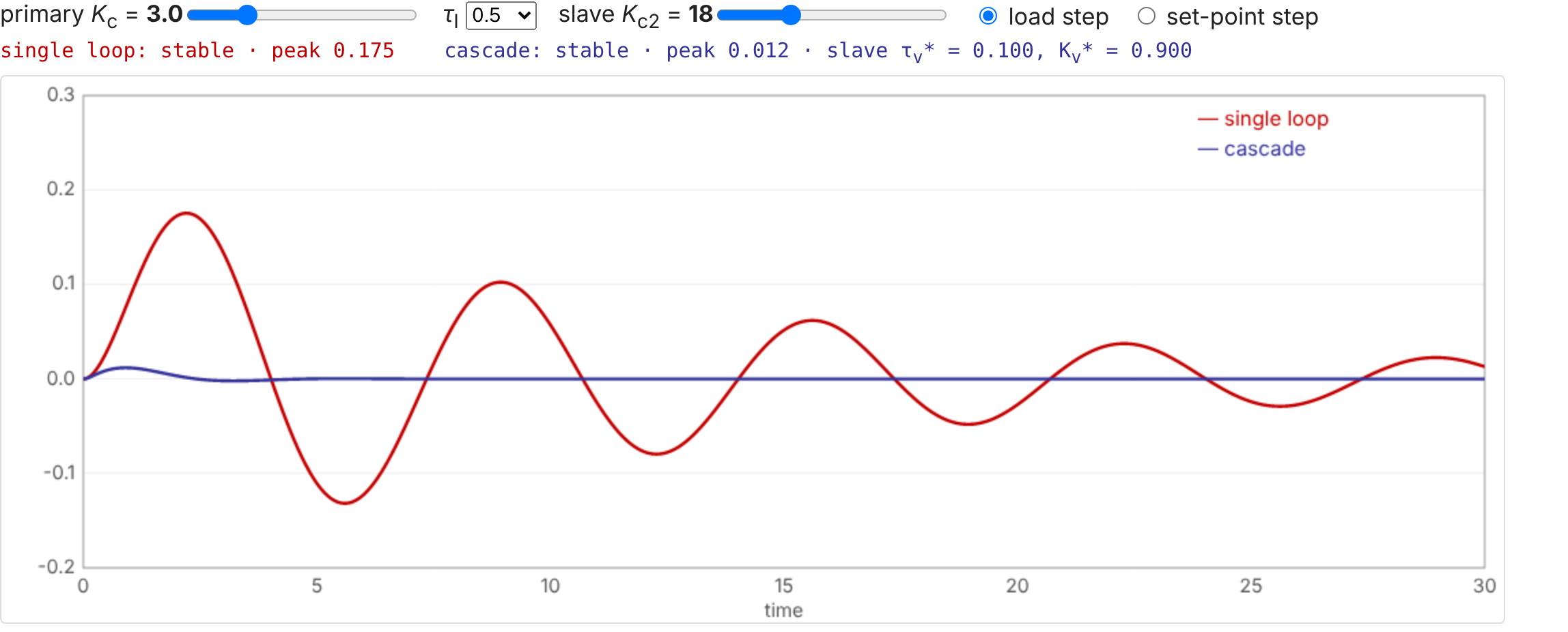
With the same master tuning (\(K_c=3,\ \tau_I=0.5\)), a fuel-gas pressure upset moves the temperature 15× less with the cascade (peak 0.175 → 0.012). The set-point response is also much better damped.

Example 6.1 in code

import numpy as np, control as ct

Gp, Gv, GL = ct.tf(0.8, [2, 1]), ct.tf(0.5, [1, 1]), ct.tf(0.75, [1, 1])
Kc2 = 18
Gv_s = ct.feedback(Kc2*Gv, 1)                   # G_v*  = 9/(s+10)
GL_s = ct.minreal(GL/(1 + Kc2*Gv))              # G_L*  = 0.75/(s+10)

Kc, tI = 3, 0.5
Gc = ct.tf([Kc*tI, Kc], [tI, 0])
load_single  = ct.minreal(GL*Gp/(1 + Gc*Gv*Gp))
load_cascade = ct.minreal(GL_s*Gp/(1 + Gc*Gv_s*Gp))
t = np.linspace(0, 30, 3001)
for T in (load_single, load_cascade):
    print(ct.step_response(T, t).outputs.max())   # 0.175, 0.012
Gp = tf(0.8,[2 1]);  Gv = tf(0.5,[1 1]);  GL = tf(0.75,[1 1]);
Kc2 = 18;
Gv_s = feedback(Kc2*Gv, 1);                % G_v*
GL_s = minreal(GL/(1 + Kc2*Gv));           % G_L*

Kc = 3;  tI = 0.5;  Gc = Kc*tf([tI 1],[tI 0]);
load_single  = minreal(GL*Gp/(1 + Gc*Gv*Gp));
load_cascade = minreal(GL_s*Gp/(1 + Gc*Gv_s*Gp));
step(load_single, load_cascade, 30), legend('single loop','cascade')

6.2 Feedforward Control

Act on the disturbance, not on the error

Measure the disturbance \(L\) and use a process model to move \(M\) before \(C\) is affected:

\[ C=G_LL+G_pM\quad\xrightarrow{\;C=R\;}\quad M=\frac{1}{G_p}R-\frac{G_L}{G_p}L \]

  • Set-point changes are normally left to the feedback loop; only the second term is implemented.
  • The feedforward controller is the model-based rule \(-G_L/G_p\).
Gc​ + + Gv​*​ Gp​ + + GmL​ GFF​ GL​ M C L measured disturbance feedback loop (added in §6.3) feedforward: acts before C moves

The feedforward controller

\[ C=\big[G_L+G_{mL}G_{FF}G_v^*G_p\big]L \;\xrightarrow{\;C=0\;}\; G_{FF}=-\frac{G_L}{G_{mL}G_v^*G_p} \]

FIX (the original wrote \(F_{FF}\) for \(G_{FF}\))

Pitfalls of the ideal \(G_{FF}\):

  • often not realizable: the numerator order exceeds the denominator order
  • a dead time in \(G_p\) larger than in \(G_L\) gives \(e^{+\theta s}\), which would need the future
  • it is only as good as the model

Practical form: lead-lag × gain

\[ G_{FF}=K_{FF}\,\frac{\tau_{ld}s+1}{\tau_{lg}s+1} \] \[ K_{FF}=-\frac{K_L}{K_{mL}K_v^*K_p} \]

  • static part \(K_{FF}\): steady-state compensator
  • lead-lag: dynamic compensator

If the measurement is fast and \(\tau_v^*\) is small (a cascade slave loop), the static gain alone may be enough — but check (Ex 6.7).

Example 6.7   Static or dynamic feedforward? NEW
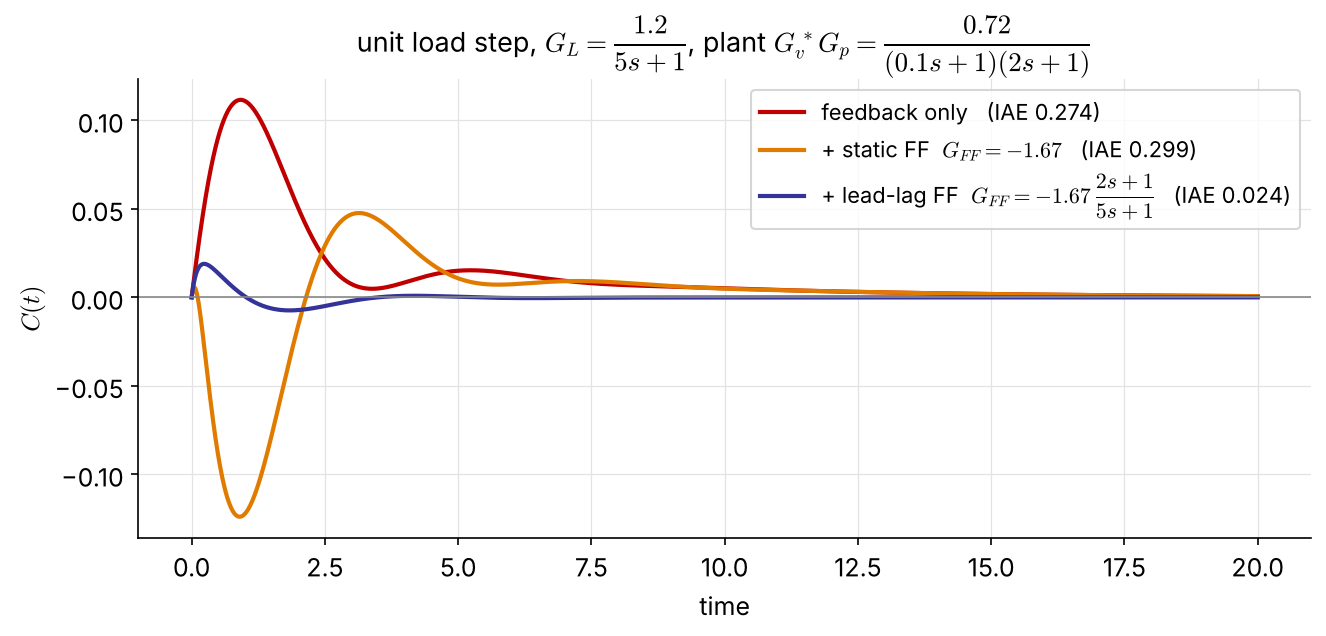
Cascade plant of Ex 6.1 with a load at the output: \(G_L=\dfrac{1.2}{5s+1}\), \(\ G_{mL}=1\), PI \(K_c=3,\ \tau_I=0.5\)

\[ G_{FF}^{\text{ideal}}=-1.67\,\frac{(0.1s+1)(2s+1)}{5s+1} \] improper → drop the fast \((0.1s+1)\): \[ G_{FF}=-1.67\,\frac{2s+1}{5s+1} \]

The static \(G_{FF}\) acts too early (the load is slower than the process) and makes things worse than feedback alone. The lead-lag cuts IAE 11×.

6.3 Feedforward–Feedback Control

Feedforward never works alone

R + − E Gc​ + + Gv​*​ Gp​ + + GmL​ GFF​ GL​ M C L measured disturbance Gm​ feedback: corrects model error feedforward: acts before C moves

\[ C=\frac{G_L+G_{mL}G_{FF}G_v^*G_p}{1+G_mG_cG_v^*G_p}\,L+\frac{G_cG_v^*G_p}{1+G_mG_cG_v^*G_p}\,R \]

Characteristic equation \(1+G_mG_cG_v^*G_p=0\): \(G_{FF}\) does not affect stability.

Feedforward does most of the work; feedback removes what the imperfect model leaves behind.

Example 6.2   Furnace with feedforward, feedback and cascade

furnace cold process stream hot process stream T TT TC Ts​ fuel gas FT FC Σ TT FT FFC inlet T inlet flow feedforward signal FB + FF → FC set point

Inlet temperature and flow of the process stream (the main loads) feed the FFC; its signal is added (Σ) to the TC output. The sum is the set point of the fuel-gas flow controller, so cascade handles the fuel-supply upsets.

6.4 Ratio Control

Keeping air in proportion to fuel

(a) simple ratio control fuel gas (wild stream) FFG​ FT RS ratio station FA​s​ = R FFG​ FC air FA​ FT (b) full-metering ratio control Σ set point from the FF–FB loops FC fuel gas → furnace FT RC R FC air → furnace FT

(a) Simple ratio: the fuel flow is “wild” (set elsewhere). The ratio station RS multiplies its measurement by \(R=F_A/F_{FG}\) to give the air-flow set point.

(b) Full metering: both flows are controlled. The fuel set point comes from the FF–FB loops, and the ratio controller RC sets the air flow from the measured fuel flow.

6.5 The Smith Predictor

Dead time in the loop

\[ 1+G_c(s)G(s)e^{-\theta s}=0 \]

  • Dead time adds phase lag \(-\omega\theta\), lowers the gain margin, and forces a small \(K_c\) (Ch 5).
  • The root cause is that the measured output is outdated information.

If \(G(s)\) and \(\theta\) are known, predict the undelayed output and feed that back instead.

Notation: the original slides use \(t_d\); here \(\theta\), as in Ch 4–5.

The Smith predictor

(a) feedback with dead time R + − Gc​(s) G(s)e−θs​ Y 1 + Gc​Ge−θs​ = 0: delay in the loop (b) Smith predictor (dead-time compensator) R + − − Gc​(s) G(s)e−θs​ G(s)(1 − e−θs​) E Y (c) equivalent loop R + − Gc​ G e−θs​ Y delay moved outside the loop char. eq. 1 + Gc​G = 0

\[ E=R-Y-G_cG\left(1-e^{-\theta s}\right)E,\qquad Y=G_cGe^{-\theta s}E \] \[ \Rightarrow\;E=R-G_cG\,E,\qquad \frac{Y}{R}=\frac{G_cG}{1+G_cG}\,e^{-\theta s} \]

The characteristic equation \(1+G_cG=0\) has no dead time. Tune \(G_c\) as if the delay were absent; the response is the same, only shifted by \(\theta\). NEW

Example 6.8   Smith predictor on the Ex 4.4 plant NEW
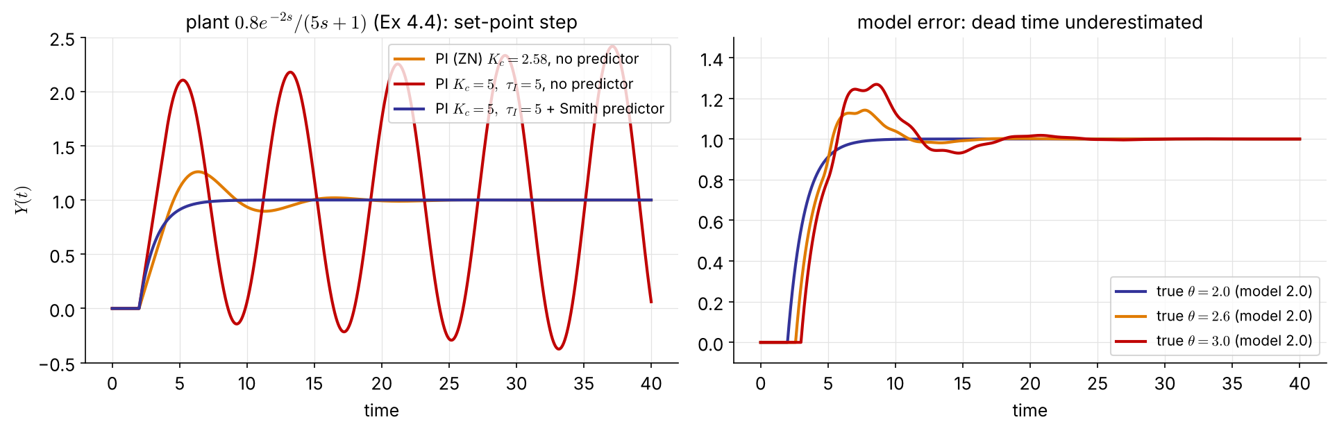
\(G=\dfrac{0.8e^{-2s}}{5s+1}\), \(\ K_{cu}=5.73\) (Ch 4–5). PI with \(\tau_I=5\) cancels the lag, and \(K_c=5\) gives a first-order loop with \(\tau_{cl}=5/(0.8K_c)=1.25\).

  • without the predictor, \(K_c=5\) is unstable
  • with it: no overshoot, \(Y(t)\) is the ideal response delayed by 2

Caveats: it needs an accurate model; a 50 % dead-time error brings back overshoot. For load disturbances the delay is not removed; the predictor only speeds up the correction.

Smith predictor in code

from blocks import FOPDT, Delay, PI, DT     # exact dead time (no Pade); blocks.py in ch6/
import numpy as np

def smith(Kc, tI, theta_true=2.0, theta_model=2.0, tf=40):
    G  = FOPDT(0.8, 5, theta_true)           # plant  0.8 e^{-theta s}/(5s+1)
    M0 = FOPDT(0.8, 5, 0.0)                  # model without delay
    Md = Delay(theta_model)                  # model delay
    c  = PI(Kc, tI)
    y = ym0 = ymd = 0.0; out = []
    for k in range(int(tf/DT) + 1):
        u = c(1.0 - y - (ym0 - ymd))         # feed back y + G(1 - e^{-theta s}) u
        y, ym0 = G(u), M0(u); ymd = Md(ym0)
        out.append(y)
    return np.arange(len(out))*DT, np.array(out)

t, y = smith(5, 5)                           # Kc = 5 > Kcu: still stable
s  = tf('s');
G0 = 0.8/(5*s + 1);                  % model without delay
Gd = ss(G0*exp(-2*s));               % plant with delay (ss: internal delays)
Gc = 5*(1 + 1/(5*s));                % PI, Kc = 5, tauI = 5

C_smith = feedback(Gc, G0 - Gd);     % controller + dead-time compensator
T_smith = feedback(C_smith*Gd, 1);   % = Gc*G0/(1+Gc*G0) * exp(-2s)
T_plain = feedback(Gc*Gd, 1);        % unstable
step(T_smith, 40)

6.6 Multiple-Input Multiple-Output Control

A blending process

m1​ pure A m2​ solvent FT CT FC CC F x control total flow F and composition x with the two valve flows m1​, m2​ G11​ G12​ G21​ G22​ + + + + M1​ M2​ C1​ = x C2​ = F

\[ C_1=G_{11}M_1+G_{12}M_2,\qquad C_2=G_{21}M_1+G_{22}M_2 \]

Every manipulated variable affects both outputs. The questions are: which \(M\) should control which \(C\), and how strongly do the loops fight?

MIMO closed loop

R1​ + − R2​ + − Gc1​ Gc2​ M1​ M2​ G11​ G12​ G21​ G22​ + + + + C1​ C2​

With \(M_i=G_{ci}(R_i-C_i)\), the closed loop is

\[ \begin{bmatrix}C_1\\C_2\end{bmatrix}=\frac{1}{p(s)} \begin{bmatrix}G_{11}G_{c1}+g(s) & G_{12}G_{c2}\\ G_{21}G_{c1} & G_{22}G_{c2}+g(s)\end{bmatrix} \begin{bmatrix}R_1\\R_2\end{bmatrix},\qquad g=(G_{11}G_{22}-G_{12}G_{21})G_{c1}G_{c2} \]

\(p(s)=(1+G_{11}G_{c1})(1+G_{22}G_{c2})-G_{12}G_{21}G_{c1}G_{c2}=0\): tuning one loop changes the stability of both.

Process gain matrix

Mass balances (\(m_1\) pure A, \(m_2\) solvent): \(\;F=m_1+m_2,\quad x=\dfrac{m_1}{m_1+m_2}\)

\[ x\approx x_s+\underbrace{\left[\frac{m_2}{(m_1+m_2)^2}\right]_s}_{K_{11}}(m_1-m_{1,s})\;\underbrace{-\left[\frac{m_1}{(m_1+m_2)^2}\right]_s}_{K_{12}}(m_2-m_{2,s}) \]

\[ \begin{bmatrix}X\\F\end{bmatrix}=\underbrace{\begin{bmatrix}K_{11}&K_{12}\\K_{21}&K_{22}\end{bmatrix}}_{\mathbf K}\begin{bmatrix}M_1\\M_2\end{bmatrix},\quad K_{21}=K_{22}=1 \]

Example 6.3   \(m_1=0.1,\ m_2=10\) g/s: \[ \mathbf K=\begin{bmatrix}9.8\times10^{-2} & -9.8\times10^{-4}\\ 1 & 1\end{bmatrix} \] \(|K_{11}|\gg|K_{12}|\): \(m_2\) barely affects \(x\), a nearly one-way interaction.

Relative gain array (RGA)

\[ \lambda_{ij}=\frac{\left.\dfrac{\partial c_i}{\partial m_j}\right|_{m_k,\,k\neq j}}{\left.\dfrac{\partial c_i}{\partial m_j}\right|_{c_k,\,k\neq i}} =\frac{\text{gain with all other loops open}}{\text{gain with all other loops closed (perfect control)}} \]

For a \(2\times2\) system, with \(\kappa=\dfrac{K_{12}K_{21}}{K_{11}K_{22}}\):

\[ \lambda_{11}=\frac{1}{1-\kappa},\qquad \boldsymbol\Lambda=\begin{bmatrix}\lambda_{11}&1-\lambda_{11}\\1-\lambda_{11}&\lambda_{11}\end{bmatrix} \]

Properties NEW

  • each row and column sums to 1
  • independent of the units and scaling of the variables
  • any size: \(\;\boldsymbol\Lambda=\mathbf K\circ\left(\mathbf K^{-1}\right)^{T}\) (element-wise product)

Example 6.4   RGA of the blending process

\[ \left.\frac{\partial x}{\partial m_1}\right|_{m_2}=\frac{m_2}{(m_1+m_2)^2},\qquad \left.\frac{\partial x}{\partial m_1}\right|_{F}=\frac{1}{F}=\frac{1}{m_1+m_2} \;\Rightarrow\; \lambda_{x,m_1}=\frac{m_2}{m_1+m_2}=1-x \]

\[ \boldsymbol\Lambda=\begin{bmatrix}\lambda_{x,m_1}&\lambda_{x,m_2}\\\lambda_{F,m_1}&\lambda_{F,m_2}\end{bmatrix}=\begin{bmatrix}1-x&x\\x&1-x\end{bmatrix} \]

Same result from the gains: \(\kappa=K_{12}K_{21}/(K_{11}K_{22})=-m_1/m_2\)
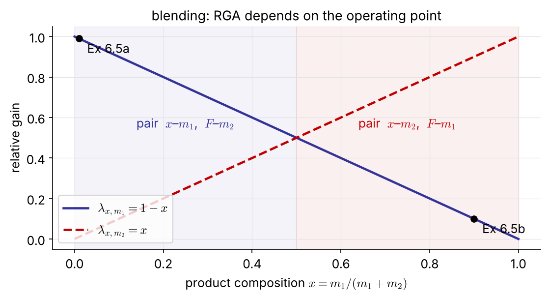
Reading the RGA: pairing rules FIX

\(\lambda_{ij}\) \(\kappa\) (2×2) meaning pair \(m_j\)–\(c_i\)?
\(1\) \(0\) no interaction from the other loop yes, ideal
\(0.5\)–\(1\) \(<0\) closing the other loop raises this loop’s gain yes
\(>1\) \(0\)–\(1\) closing the other loop lowers the gain yes; avoid \(\lambda\gg1\)
\(0.5\) \(-1\) the other loop doubles the gain; both pairings bad —
\(0\) — \(m_j\) has no effect on \(c_i\) no
\(<0\) \(>1\) the gain changes sign when the other loop closes never

Example 6.5   Pairing depends on the operating point

(a) \(m_1=0.1,\ m_2=10\) g/s (\(x=0.0099\)) \[ \boldsymbol\Lambda=\begin{bmatrix}\mathbf{0.9901}&0.0099\\0.0099&\mathbf{0.9901}\end{bmatrix} \] pair \(x\)–\(m_1\), \(F\)–\(m_2\)

(b) \(m_1=9,\ m_2=1\) g/s (\(x=0.9\)) \[ \boldsymbol\Lambda=\begin{bmatrix}0.1&\mathbf{0.9}\\\mathbf{0.9}&0.1\end{bmatrix} \] pair \(x\)–\(m_2\), \(F\)–\(m_1\)

Control the composition with the smaller stream: it changes \(x\) more and \(F\) less.

RGA in code

import numpy as np

def rga(K):
    K = np.asarray(K, float)
    return K * np.linalg.inv(K).T            # Lambda = K o (K^-1)^T

m1, m2 = 0.1, 10.0; F = m1 + m2
K = [[m2/F**2, -m1/F**2],
     [1.0,      1.0    ]]
print(rga(K))                                # [[0.9901 0.0099] [0.0099 0.9901]]

K66 = [[0.07, -0.05], [0.1, -0.15]]          # distillation, Ex 6.6
print(rga(K66))                              # [[ 1.91 -0.91] [-0.91  1.91]]
rga = @(K) K .* inv(K).';                    % Lambda = K o (K^-1)^T

m1 = 0.1;  m2 = 10;  F = m1 + m2;
K = [m2/F^2, -m1/F^2;
     1,       1     ];
rga(K)                                       % [0.9901 0.0099; 0.0099 0.9901]

K66 = [0.07 -0.05; 0.1 -0.15];               % distillation, Ex 6.6
rga(K66)                                     % [1.91 -0.91; -0.91 1.91]

6.7 Decoupling of Interacting Systems

Feedforward-like decouplers

R1​ + − R2​ + − Gc1​ Gc2​ + + + + D21​ D12​ M1​ M2​ G11​ G12​ G21​ G22​ + + + + C1​ C2​

Cancel the effect of controller 2 on \(C_1\): \[ G_{12}+G_{11}D_{12}=0\;\Rightarrow\;D_{12}=-\frac{G_{12}}{G_{11}} \]

Cancel the effect of controller 1 on \(C_2\): \[ G_{21}+G_{22}D_{21}=0\;\Rightarrow\;D_{21}=-\frac{G_{21}}{G_{22}} \]

Example 6.6   Distillation column

\[ \begin{bmatrix}X_D\\X_B\end{bmatrix}= \begin{bmatrix}\dfrac{0.07e^{-3s}}{12s+1}&\dfrac{-0.05e^{-s}}{15s+1}\\[2mm]\dfrac{0.1e^{-4s}}{11s+1}&\dfrac{-0.15e^{-2s}}{10s+1}\end{bmatrix} \begin{bmatrix}L\\V\end{bmatrix} \qquad L:\text{ reflux},\ V:\text{ boil-up} \]

\[ \mathbf K=\begin{bmatrix}0.07&-0.05\\0.1&-0.15\end{bmatrix} \] \[ \boldsymbol\Lambda=\begin{bmatrix}1.91&-0.91\\-0.91&1.91\end{bmatrix} \]

Pair \(x_D\)–\(L\), \(x_B\)–\(V\): \(\lambda=1.91\) is not 1 but it is positive, and the reflux enters next to the distillate.

Decouplers \[ D_{12}=-\frac{G_{12}}{G_{11}}=0.714\,\frac{12s+1}{15s+1}\,e^{+2s}\approx0.71 \] \[ D_{21}=-\frac{G_{21}}{G_{22}}=0.667\,\frac{10s+1}{11s+1}\,e^{-2s}\approx0.67 \] \(D_{12}\) would need a prediction (\(e^{+2s}\)) → drop it; \(D_{21}\) is realizable as it stands. NEW

Example 6.6: PI tuning (ITAE)

ITAE set-point correlations for FOPDT loops, applied to the diagonal elements: \(\;K_c=\dfrac{0.586}{K}\left(\dfrac{\theta}{\tau}\right)^{-0.916},\quad \tau_I=\dfrac{\tau}{1.03-0.165\,\theta/\tau}\)

\[ K_{c1}=\frac{0.586}{0.07}\left(\frac{12}{3}\right)^{0.916}=29.8 \] \[ \tau_{I1}=\frac{12}{1.03-0.165(3/12)}=12.1 \]

\[ K_{c2}=-\frac{0.586}{0.15}\left(\frac{10}{2}\right)^{0.916}=-17.1 \] \[ \tau_{I2}=\frac{10}{1.03-0.165(2/10)}=10.0 \]

Example 6.6: does decoupling help? (replaces the Simulink runs)
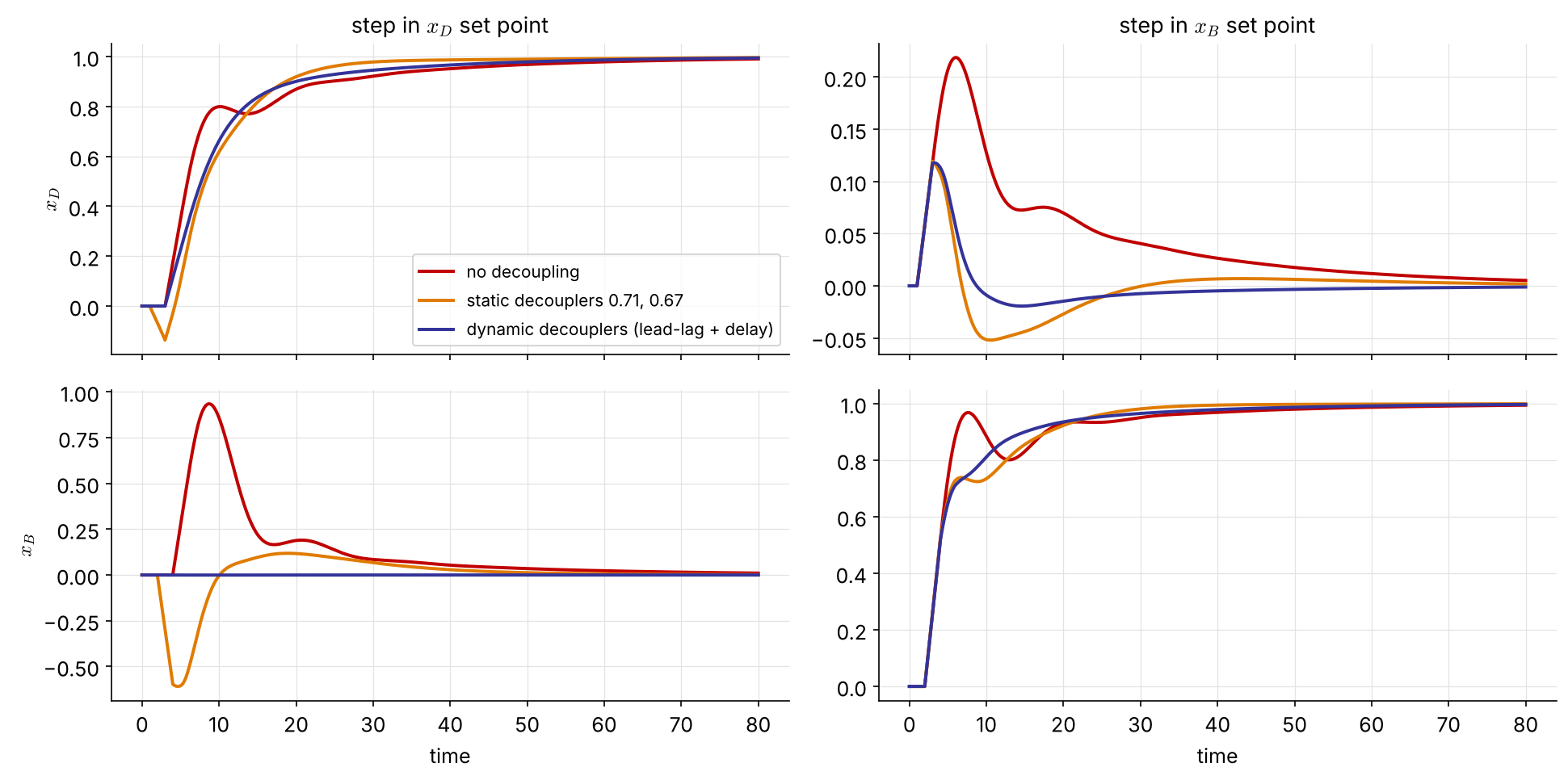
  • No decoupling: an \(x_D\) set-point step drives \(x_B\) up to 0.94.
  • Static decouplers: \(x_B\) now dips to \(-0.61\). \(D_{21}\) acts at \(t=2\) through \(G_{22}\), before \(G_{21}\) arrives at \(t=4\).
  • Dynamic \(D_{21}\) (with its \(e^{-2s}\)): \(x_B\) stays at 0, exact decoupling. NEW

A decoupler that ignores the timing can trade one interaction for another. Keep realizable delays and lags.

Decoupling in code

from blocks import simulate_2x2              # exact dead time; blocks.py in ch6/

G = [[(0.07, 12, 3), (-0.05, 15, 1)],        # (K, tau, theta) of each G_ij
     [(0.10, 11, 4), (-0.15, 10, 2)]]
Kc = (29.8, -17.1);  tI = (12.1, 10.0)

cases = {'none':    (None, None),
         'static':  (0.714, 0.667),
         'dynamic': ((0.714, 12, 15, 0), (0.667, 10, 11, 2))}   # (K, tau_lead, tau_lag, theta)
for name, (D12, D21) in cases.items():
    t, xD, xB, L, V = simulate_2x2(G, Kc, tI, D12, D21, r1=1, r2=0, tf=80)
    print(name, 'max |x_B| =', abs(xB).max().round(2))     # 0.93, 0.61, 0.00
s = tf('s');
G = [0.07*exp(-3*s)/(12*s+1), -0.05*exp(-s)/(15*s+1);
     0.10*exp(-4*s)/(11*s+1), -0.15*exp(-2*s)/(10*s+1)];
C = blkdiag(29.8*(1 + 1/(12.1*s)), -17.1*(1 + 1/(10.0*s)));

D_static  = [1, 0.714; 0.667, 1];                          % M = D * u
D_dynamic = [1, 0.714*(12*s+1)/(15*s+1);
             0.667*(10*s+1)/(11*s+1)*exp(-2*s), 1];
for D = {eye(2), D_static, D_dynamic}
    T = feedback(ss(G)*D{1}*C, eye(2));               % ss: mixed delays
    step(T(:,1), 80), hold on                              % step in r1 (x_D)
end

Interactive: cascade vs. single loop NEW
Summary: which structure for which problem?

Symptom Structure Needs
upsets enter through the manipulated stream cascade a secondary measurement much faster than the primary
a large disturbance can be measured feedforward + feedback a model of \(G_L/G_p\) (lead-lag is usually enough)
two streams must stay proportional ratio flow measurements
dead time dominates Smith predictor an accurate model, especially of \(\theta\)
several loops interact RGA pairing, then decoupling gain matrix (pairing); dynamic model (decoupling)

Problem #1   (homework) NEW

\[ \mathbf G(s)=\begin{bmatrix}\dfrac{2e^{-s}}{10s+1} & \dfrac{1.5e^{-s}}{15s+1}\\[2mm] \dfrac{1.5e^{-s}}{15s+1} & \dfrac{2e^{-s}}{10s+1}\end{bmatrix} \]

  1. Compute the RGA. Which pairing do you choose, and how strong is the interaction?

  2. Design the two decouplers. Are they realizable? Compare the static and dynamic versions.

  3. Tune two PI controllers with the ITAE correlations and simulate a step in \(R_1\) with and without decoupling (use simulate_2x2 from blocks.py).

Resources

Further reading:

  • D. E. Seborg, T. F. Edgar, D. A. Mellichamp, Process Dynamics and Control
  • P. C. Chau, Process Control: A First Course with MATLAB
  • B. W. Bequette, Process Control: Modeling, Design, and Simulation
  • C. D. Johnson, Process Control Instrumentation Technology
  • S. Skogestad, I. Postlethwaite, Multivariable Feedback Control: Analysis and Design

A final word — Neal R. Amundson (University of Minnesota, circa 1970)

  1. In an advanced course … when has any substance there will be no text which contains all of the material presented.
  2. Teachers who know their subject well will always present material not in the prescribed text when one is prescribed.
  3. If there were a text which presented all of the materials there would be no need for the lecturer.
  4. In a course of any substance it will not be possible for the student to understand or follow all of the arguments instantaneously all of the time.
  5. Assuming that 4 is true it is essential that good notes be taken. Usually this is not possible. Normally the notes will be very sketchy and if they are to be of any use later, they must be expanded upon by the student as soon after the lecture as possible.
  6. Because of 5 notes in real courses must be recopied, filled out, corrected for teacher aberrations, misprints, errors, etc., so that the student ends up with his own text.
  1. Notes which have not been so treated are normally almost useless for later reference.
  2. In core subjects one must learn and memorize and in this way make deposits in the bank from which he can withdraw later. If nothing is ever put in the bank then one is intellectually bankrupt. All knowledge is what one knows. If one cannot verbalize what he knows then he properly does not understand what he thinks he knows.
  3. First-year graduate students, in general, must change their ways of studying from their undergraduate habits since in respectable graduate programs the emphasis is on understanding rather than getting through the course. This necessary shift is why many first-year graduate students go into shock after about six weeks of graduate work.
  4. If a student aims toward a Ph.D. degree he is expected not only to understand but be able to improve by generalization or better by innovations. Good graduate programs require the latter.
  5. 10 is what research is all about.
