3. Tuning of Single-Loop Control Systems
A PID controller needs only three numbers, \(K_c\), \(\tau_I\) and \(\tau_D\), yet choosing them is one of the most confusing parts of learning control.
Different tuning techniques give similar but not identical results. There is no “best” or “absolutely correct” answer, only trade-offs between speed, overshoot and robustness.
| Approach | Experiment | Model | Methods |
|---|---|---|---|
| Empirical (3.1) | open-loop step test | FOPDT fit \(\dfrac{Ke^{-\theta s}}{\tau s+1}\) | Ziegler–Nichols, Cohen–Coon, ITAE |
| closed-loop test | \(K_{cu}\), \(T_u\) only | ZN ultimate cycle | |
| Model-based (3.2) | — | transfer function | direct synthesis, IMC |
The settings are a quick-and-dirty starting point. They are seldom optimal and usually need field tuning after installation to meet the actual response specifications.
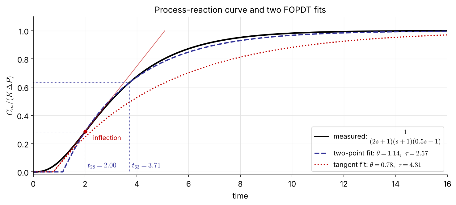
With the controller disconnected, step the controller output by \(P=M/s\) and record the measured output. What we see is the lumped response of valve, process and sensor:
\[ G_{PRC}=\frac{C_m}{P}=G_aG_pG_m\;\approx\;\frac{Ke^{-\theta s}}{\tau s+1} \]
Two-point method (Smith): read \(t_{28}\) and \(t_{63}\) at 28.3 % and 63.2 % of the final change \[ \tau=1.5\,(t_{63}-t_{28}),\qquad \theta=t_{63}-\tau,\qquad K=\frac{\Delta C_m}{\Delta P} \]
Tangent method: draw the tangent at the inflection point. Its intercepts give \(\theta\) and \(\tau\).
Simple, but it overestimates \(\tau\) and underestimates \(\theta\), so it gives aggressive settings.
| Controller | Cohen–Coon | Ziegler–Nichols | |
|---|---|---|---|
| P | \(K_cK\) | \(\dfrac{\tau}{\theta}+\dfrac13\) | \(\dfrac{\tau}{\theta}\) |
| PI | \(K_cK\) | \(0.9\dfrac{\tau}{\theta}+\dfrac{1}{12}\) | \(0.9\dfrac{\tau}{\theta}\) |
| \(\tau_I\) | \(\theta\,\dfrac{30+3\theta/\tau}{9+20\theta/\tau}\) | \(3.3\,\theta\) | |
| PID | \(K_cK\) | \(\dfrac43\dfrac{\tau}{\theta}+\dfrac14\) | \(1.2\dfrac{\tau}{\theta}\) |
| \(\tau_I\) | \(\theta\,\dfrac{32+6\theta/\tau}{13+8\theta/\tau}\) | \(2\,\theta\) | |
| \(\tau_D\) | \(\theta\,\dfrac{4}{11+2\theta/\tau}\) | \(0.5\,\theta\) |
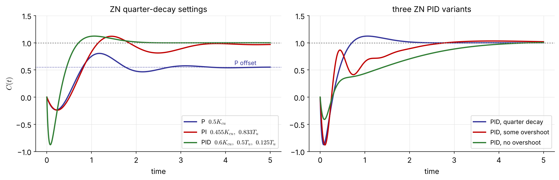
Both aim at a quarter-decay ratio, which is fast but oscillatory. Note \(K_c\propto 1/K\) and \(K_c\propto\tau/\theta\): the larger the dead time relative to the time constant, the gentler the controller.
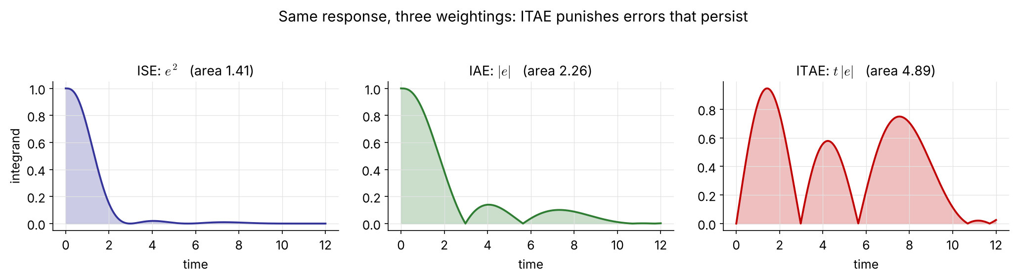
\[ \mathrm{ISE}=\int_0^\infty e^2(t)\,dt \] \[ \mathrm{IAE}=\int_0^\infty |e(t)|\,dt \] \[ \mathrm{ITAE}=\int_0^\infty t\,|e(t)|\,dt \]
Load change \[ K_c=\frac{a_1}{K}\left(\frac{\tau}{\theta}\right)^{b_1},\quad \tau_I=\frac{\tau}{a_2}\left(\frac{\theta}{\tau}\right)^{b_2} \]
| \(a_1\) | \(b_1\) | \(a_2\) | \(b_2\) | \(a_3\) | \(b_3\) | |
|---|---|---|---|---|---|---|
| PI | 0.859 | 0.977 | 0.674 | 0.680 | — | — |
| PID | 1.357 | 0.947 | 0.842 | 0.738 | 0.381 | 0.995 |
Set-point change \[ K_c=\frac{a_1}{K}\left(\frac{\tau}{\theta}\right)^{b_1},\quad \tau_I=\frac{\tau}{a_2-b_2\,\theta/\tau} \]
| \(a_1\) | \(b_1\) | \(a_2\) | \(b_2\) | \(a_3\) | \(b_3\) | |
|---|---|---|---|---|---|---|
| PI | 0.586 | 0.916 | 1.03 | 0.165 | — | — |
| PID | 0.965 | 0.855 | 0.796 | 0.147 | 0.308 | 0.929 |
\[ \text{both:}\qquad \tau_D=a_3\,\tau\left(\frac{\theta}{\tau}\right)^{b_3} \]
Load settings are more aggressive (higher \(K_c\), shorter \(\tau_I\)) than set-point settings. Choose the table for the disturbance you expect most.
For processes that are open-loop stable but can be destabilized by feedback.
These are exactly the \(K_{cu}\) and \(\omega_u=2\pi/T_u\) of Ch 4 (Routh, direct substitution) and Ch 5 (gain margin).
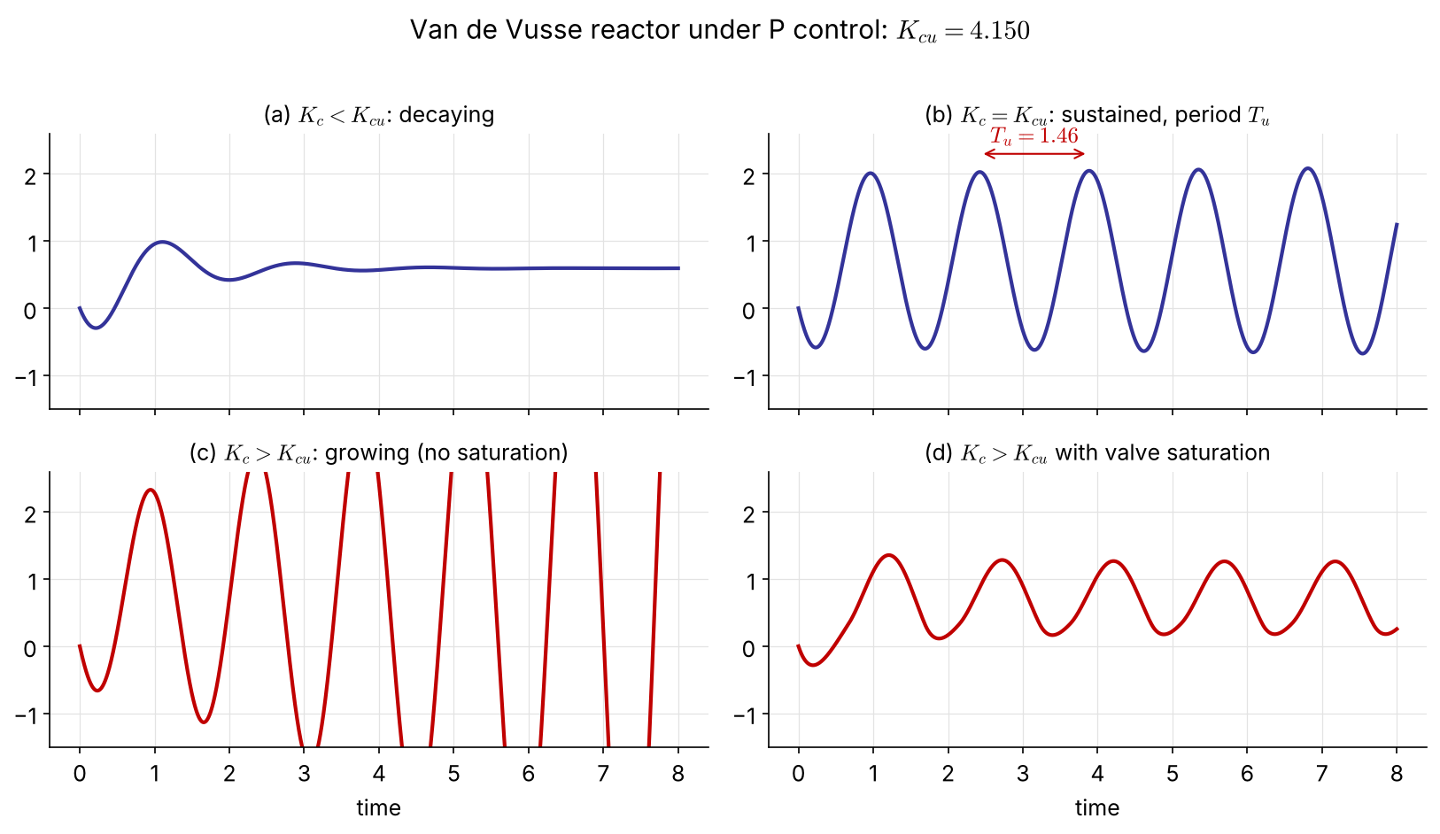
With valve saturation (d) the oscillation stays bounded and looks sustained even above \(K_{cu}\), so check that the valve is not hitting its limits.
| Controller | \(K_c\) | \(\tau_I\) | \(\tau_D\) | |
|---|---|---|---|---|
| P | \(0.5\,K_{cu}\) | — | — | |
| PI | \(0.455\,K_{cu}\) | \(0.833\,T_u\) | — | |
| PID | quarter decay | \(0.6\,K_{cu}\) | \(0.5\,T_u\) | \(0.125\,T_u\) |
| some overshoot | \(0.33\,K_{cu}\) | \(0.5\,T_u\) | \(0.333\,T_u\) | |
| no overshoot | \(0.2\,K_{cu}\) | \(0.5\,T_u\) | \(0.333\,T_u\) |
Advantages: no model is needed, and the test is done on the real loop. Drawbacks: the plant is pushed to the edge of instability, and it takes time.
\[ G_p(s)=\frac{0.5858\,(-0.3549s+1)}{0.1858s^2+0.8627s+1}\qquad\text{(RHP zero: inverse response)} \]
Raising \(K_c\) under P control (ultimate-cycle figure, two slides back):
\[ K_{cu}=4.150,\qquad T_u=1.46 \] FIX (the original read \(T_u=1.45\) off the plot; exact: \(\omega_u=4.297\), \(T_u=2\pi/\omega_u=1.462\))
| \(K_c\) | \(\tau_I\) | \(\tau_D\) | |
|---|---|---|---|
| P | 2.07 | — | — |
| PI | 1.89 | 1.22 | — |
| PID | 2.49 | 0.73 | 0.18 |
import numpy as np, control as ct
from tuning import pid_tf # ideal PID with filtered derivative (alpha = 0.1)
Gp = ct.tf(0.5858*np.array([-0.3549, 1]), [0.1858, 0.8627, 1])
Kcu, _, wu, _ = ct.margin(Gp) # 4.150 — no trial and error needed
Tu = 2*np.pi/wu # 1.462
settings = {'P': (0.5*Kcu,),
'PI': (0.455*Kcu, 0.833*Tu),
'PID': (0.6*Kcu, 0.5*Tu, 0.125*Tu)}
t = np.linspace(0, 5, 2001)
for name, pars in settings.items():
T = ct.feedback(pid_tf(*pars)*Gp, 1)
plt.plot(t, ct.step_response(T, t).outputs, label=name)Gp = tf(0.5858*[-0.3549 1], [0.1858 0.8627 1]);
[Kcu, ~, wu] = margin(Gp); Tu = 2*pi/wu; % 4.150, 1.462
C_P = 0.5*Kcu;
C_PI = pidstd(0.455*Kcu, 0.833*Tu);
C_PID = pidstd(0.6*Kcu, 0.5*Tu, 0.125*Tu, 10); % N = 10 <-> alpha = 0.1
step(feedback(C_P*Gp,1), feedback(C_PI*Gp,1), feedback(C_PID*Gp,1), 5)
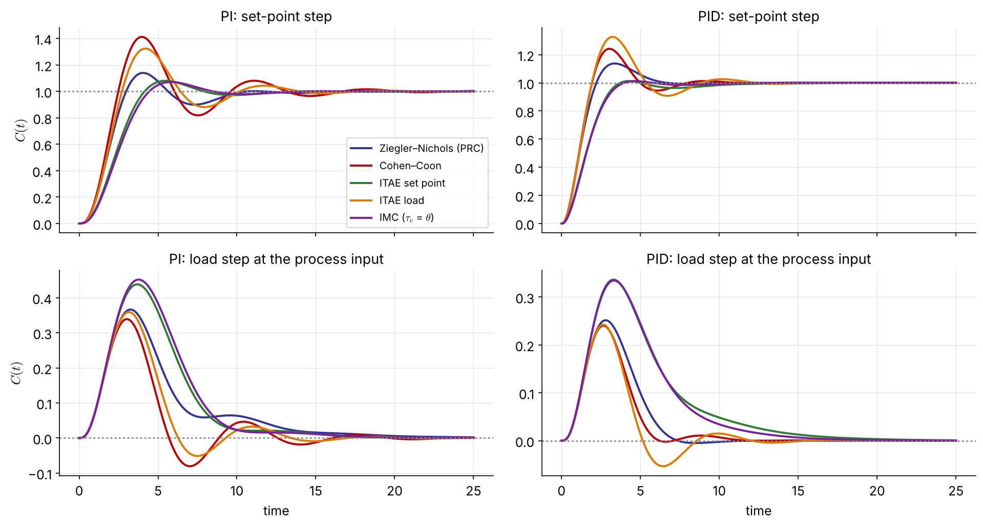
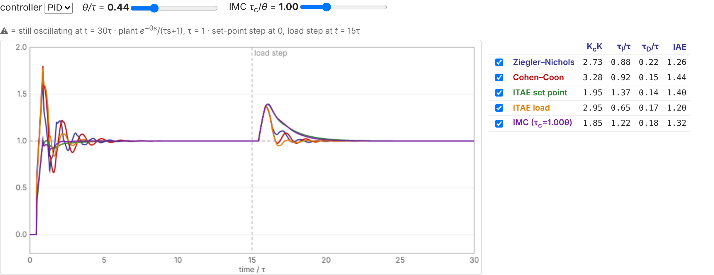
legend('P','PI','PID')“True” process \(\;\dfrac{1}{(2s+1)(s+1)(0.5s+1)}\), two-point FOPDT fit \(\;K=1,\ \tau=2.57,\ \theta=1.14\;(\theta/\tau=0.44)\)
| PID | \(K_c\) | \(\tau_I\) | \(\tau_D\) | OS | IAE sp | IAE load | GM | PM |
|---|---|---|---|---|---|---|---|---|
| Ziegler–Nichols | 2.71 | 2.28 | 0.57 | 14% | 1.48 | 0.87 | 21 | 55° |
| Cohen–Coon | 3.26 | 2.39 | 0.38 | 24% | 1.67 | 0.74 | 21 | 44° |
| ITAE set point | 1.93 | 3.52 | 0.37 | 1% | 1.84 | 1.82 | 37 | 67° |
| ITAE load | 2.93 | 1.68 | 0.44 | 33% | 2.07 | 0.81 | 23 | 38° |
| IMC, \(\tau_c=\theta\) | 1.84 | 3.14 | 0.47 | 1% | 1.74 | 1.71 | 37 | 68° |
The aggressive rules (CC, ITAE load) reject loads best and overshoot most. The gentle ones (ITAE set point, IMC) are almost overshoot-free and have twice the phase margin. No rule wins on every criterion.
import numpy as np, control as ct
from tuning import RULES, pid_tf, fit_two_point # tuning.py in ch3/
G = ct.tf(1, np.polymul(np.polymul([2, 1], [1, 1]), [0.5, 1]))
t = np.linspace(0, 30, 30001)
K, tau, theta = fit_two_point(t, ct.step_response(G, t).outputs) # 1, 2.57, 1.14
for name, rule in RULES.items():
Kc, tI, tD = rule('PID', K, tau, theta)
T = ct.feedback(pid_tf(Kc, tI, tD)*G, 1)
gm, pm, *_ = ct.margin(pid_tf(Kc, tI, tD)*G)
print(f'{name:22s} Kc={Kc:.2f} tI={tI:.2f} tD={tD:.2f} GM={gm:.1f} PM={pm:.0f}')G = tf(1, conv(conv([2 1],[1 1]),[0.5 1]));
[y, t] = step(G, 30);
t28 = t(find(y >= 0.283, 1)); t63 = t(find(y >= 0.632, 1));
tau = 1.5*(t63 - t28); theta = t63 - tau; K = y(end); % 2.57, 1.14, 1
r = theta/tau; % ITAE set point, PID
Kc = 0.965/K*(1/r)^0.855; tI = tau/(0.796 - 0.147*r); tD = 0.308*tau*r^0.929;
C = pidstd(Kc, tI, tD, 10);
figure, step(feedback(C*G, 1)), figure, margin(C*G)
Interactive version: seoultechpse.github.io/ProCon/ch3/ch3_tuning.html — vary \(\theta/\tau\), PI/PID and the IMC \(\tau_c\).
A different philosophy: specify the desired closed-loop response, then solve for the controller. The result depends on the process model, so this is a model-based design.
Servo problem (\(L=0\), \(G_m=G_a=1\)):
\[ \frac{C}{R}=\frac{G_cG_p}{1+G_cG_p}\quad\Longrightarrow\quad G_c=\frac{1}{G_p}\left(\frac{C/R}{1-C/R}\right)\qquad(3.2\text{-}1) \]
\(C/R=1\) would need infinite gain. Instead ask for a first-order response with unit gain (no offset): \[ \frac{C}{R}=\frac{1}{\tau_cs+1}\;\Rightarrow\; G_c=\frac{1}{G_p}\,\frac{1}{\tau_cs} \] (3.2-2), (3.2-3)
\(\tau_c\) is the design parameter: the closed-loop time constant. The closed-loop pole is \(s=-1/\tau_c\) whatever \(G_p\) is.
It looks like magic. In reality, saturation limits how small \(\tau_c\) can be, and there is a more serious catch (next slide).
\(G_c=1/(G_p\tau_cs)\) cancels the process: the poles of \(G_c\) are the zeros of \(G_p\). An RHP zero (Van de Vusse) gives an unstable controller, and the cancellation is internally unstable even though \(C/R\) looks fine. Dead time would need \(e^{+\theta s}\), which requires knowing the future. IMC fixes both. NEW
Dead time in the target (cannot be removed): \[ \frac{C}{R}=\frac{e^{-\theta s}}{\tau_cs+1}\qquad(3.2\text{-}4) \] \[ G_c=\frac{1}{G_p}\frac{e^{-\theta s}}{(\tau_cs+1)-e^{-\theta s}}\approx\frac{1}{G_p}\frac{e^{-\theta s}}{(\tau_c+\theta)s} \] using \(e^{-\theta s}\approx1-\theta s\) in the denominator.
Underdamped target: \[ \frac{C}{R}=\frac{1}{\tau^2s^2+2\zeta\tau s+1}\qquad(3.2\text{-}6) \] \[ G_c=\frac{1}{G_p}\,\frac{1}{\tau^2s^2+2\zeta\tau s}\qquad(3.2\text{-}7) \]
\[ G_p=\frac{K_p}{\tau_ps+1},\qquad \frac{C}{R}=\frac{1}{\tau_cs+1} \]
\[ G_c=\frac{\tau_ps+1}{K_p}\,\frac{1}{\tau_cs}=\frac{\tau_p}{K_p\tau_c}\left(1+\frac{1}{\tau_ps}\right) \]
PI controller: \(\;K_c=\dfrac{\tau_p}{K_p\tau_c},\qquad \tau_I=\tau_p\)
\(K_c\) is inversely proportional to the process gain, and a faster target (small \(\tau_c\)) means a larger gain. The integral time simply equals the process time constant.
\[ G_p=\frac{K_p}{(\tau_1s+1)(\tau_2s+1)}\quad\Rightarrow\quad G_c=\frac{(\tau_1s+1)(\tau_2s+1)}{K_p\tau_cs} \]
Ideal PID: expand the numerator and factor out \((\tau_1+\tau_2)\):
\[ G_c=\frac{\tau_1+\tau_2}{K_p\tau_c}\left[1+\frac{1}{(\tau_1+\tau_2)s}+\frac{\tau_1\tau_2}{\tau_1+\tau_2}\,s\right] \]
Series (interacting) PID, \(\tau_1>\tau_2\):
\[ G_c=\frac{\tau_1}{K_p\tau_c}\left(1+\frac{1}{\tau_1s}\right)(\tau_2s+1) \]
Same controller, two parameterizations: industrial controllers come in both forms, so check which one before entering the numbers.
(left blank in the original)
\[ G_p=\frac{K_pe^{-\theta s}}{\tau_ps+1},\qquad\frac{C}{R}=\frac{e^{-\theta s}}{\tau_cs+1}\quad(3.2\text{-}4) \]
\[ G_c\approx\frac{\tau_ps+1}{K_pe^{-\theta s}}\,\frac{e^{-\theta s}}{(\tau_c+\theta)s}=\frac{\tau_ps+1}{K_p(\tau_c+\theta)s} \]
PI controller: \(\;K_c=\dfrac{\tau_p}{K_p(\tau_c+\theta)},\qquad\tau_I=\tau_p\)
The dead time cancels exactly and acts like extra \(\tau_c\), so \(K_c\) stays finite even for \(\tau_c\to0\).
(left blank in the original)
\[ G_p=\frac{K_p}{(\tau_1s+1)(\tau_2s+1)},\qquad\frac{C}{R}=\frac{1}{\tau^2s^2+2\zeta\tau s+1}\quad(3.2\text{-}6) \]
\[ G_c=\frac{(\tau_1s+1)(\tau_2s+1)}{K_p\,s\,(\tau^2s+2\zeta\tau)}=\frac{(\tau_1s+1)(\tau_2s+1)}{K_p\,2\zeta\tau\, s\left(\dfrac{\tau}{2\zeta}s+1\right)} \]
PID with a derivative filter of time constant \(\tau/2\zeta\):
\[ K_c=\frac{\tau_1+\tau_2}{2\zeta\tau K_p},\qquad \tau_I=\tau_1+\tau_2,\qquad\tau_D=\frac{\tau_1\tau_2}{\tau_1+\tau_2} \]
The controller \(G_c^*\) runs alongside a model \(\tilde G_p\). Only the mismatch \(C-\tilde C\) (model error plus disturbance) is fed back.
\[ E=R-(C-\tilde C),\quad P=G_c^*E,\quad \tilde C=\tilde G_pP \]
\[ P=\frac{G_c^*}{1-G_c^*\tilde G_p}\,(R-C)\;\Rightarrow\; \boxed{G_c=\frac{G_c^*}{1-G_c^*\tilde G_p}}\quad(3.2\text{-}8) \] An IMC design is implemented as a conventional controller \(G_c\).
\[ C=\left[\frac{(1-G_c^*\tilde G_p)\,G_L}{1+G_c^*(G_p-\tilde G_p)}\right]L+\left[\frac{G_pG_c^*}{1+G_c^*(G_p-\tilde G_p)}\right]R \]
With a perfect model (\(\tilde G_p=G_p\)), \(C/R=G_pG_c^*\): an open-loop design, which is stable whenever \(G_p\) and \(G_c^*\) are.
Split the model so the inverse never contains an RHP zero or a dead time:
\[ \tilde G_p=\tilde G_{p+}\,\tilde G_{p-},\qquad G_c^*=\frac{1}{\tilde G_{p-}}\underbrace{\left[\frac{1}{\tau_cs+1}\right]^r}_{\text{IMC filter}},\quad r=1,2,\ldots\qquad(3.2\text{-}9) \]
Perfect model: \(\;\dfrac{C}{R}=\dfrac{\tilde G_{p+}}{(\tau_cs+1)^r}\). The non-invertible part is kept, not cancelled. Choose \(r\) so that \(G_c^*\) is proper.
\[ \tilde G_p=\frac{K_pe^{-\theta s}}{\tau_ps+1}\approx\underbrace{\frac{K_p}{(\tau_ps+1)\left(\frac{\theta}{2}s+1\right)}}_{\tilde G_{p-}}\underbrace{\left(-\frac{\theta}{2}s+1\right)}_{\tilde G_{p+}} \qquad\text{(1st-order Padé)} \]
\(r=1\): \[ G_c^*=\frac{(\tau_ps+1)\left(\frac{\theta}{2}s+1\right)}{K_p(\tau_cs+1)}\qquad(3.2\text{-}11) \] Into (3.2-8): \[ G_c=\frac{(\tau_ps+1)(\theta s+2)}{K_p(\theta+2\tau_c)\,s} \]
Ideal PID \[ K_c=\frac{1}{K_p}\,\frac{2\tau_p/\theta+1}{2\tau_c/\theta+1} \] \[ \tau_I=\tau_p+\frac{\theta}{2},\qquad \tau_D=\frac{\tau_p}{2\tau_p/\theta+1} \]
Checked symbolically in the notebook. Dropping the Padé factor in \(\tilde G_{p-}\) gives the PI of Ex 3.3.

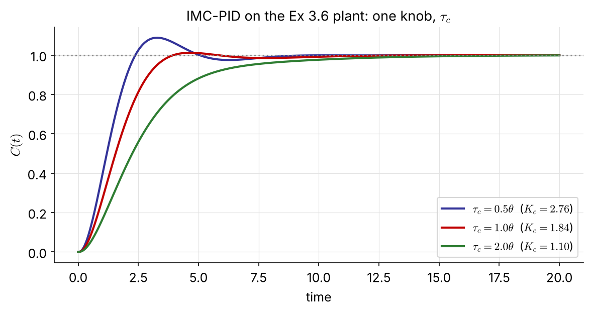
\(\tau_c\) is the single knob that trades speed for robustness:
Rule of thumb: \(\tau_c\approx\theta\). For the IMC-PI on an exact FOPDT the loop becomes \(e^{-\theta s}/(2\theta s)\): \[ \mathrm{GM}=\pi=3.1,\qquad\mathrm{PM}=61^\circ \]
\(\tilde G_{p+}=-0.3549s+1\) (RHP zero), \(\;\tilde G_{p-}=\dfrac{0.5858}{0.1858s^2+0.8627s+1}\)
\(\tilde G_{p-}\) has relative degree 2, so take \(r=2\): \[ \frac{C}{R}=\frac{-0.3549s+1}{(\tau_cs+1)^2} \] (3.2-8) gives a PID with a derivative filter: \[ G_c=\frac{0.1858s^2+0.8627s+1}{0.5858\,s\,(\tau_c^2s+2\tau_c+0.3549)} \] \(K_c=\dfrac{0.8627}{0.5858(2\tau_c+0.3549)},\ \tau_I=0.863,\ \tau_D=0.215\)
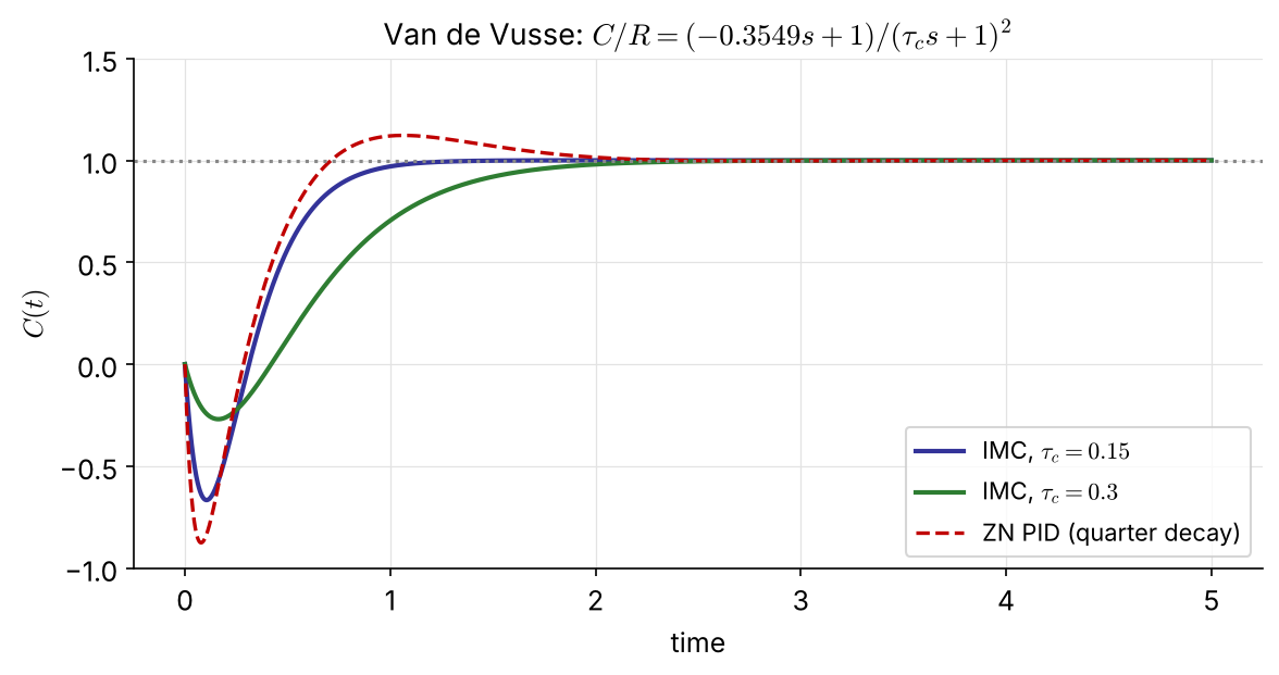
No overshoot, and \(\tau_c\) sets the depth of the inverse response: \(-0.67\) for \(\tau_c=0.15\) (\(K_c=2.25\)), \(-0.27\) for \(\tau_c=0.3\) (\(K_c=1.54\)), against \(-0.88\) for ZN PID.

| Situation | Method | Remarks |
|---|---|---|
| a step test is allowed | ZN / Cohen–Coon / ITAE from a FOPDT fit | fit by the two-point method |
| loop cannot be opened; plant tolerates cycling | ZN ultimate cycle | \(K_{cu}\), \(T_u\); Ch 4–5 compute them from a model |
| a model is available | IMC (or direct synthesis) | one physical knob \(\tau_c\); handles RHP zeros and dead time |
| robustness matters most | ITAE set point, IMC with \(\tau_c\ge\theta\) | check GM and PM (Ch 5) |
| load rejection matters most | ITAE load, Cohen–Coon | expect more overshoot on set-point changes |
Whatever the rule: verify by simulation, then field-tune.
A process stream is heated in a shell-and-tube exchanger, and \(T_2\) is controlled with the steam valve. In an open-loop test the steam pressure \(P_s\) was stepped from 18 to 20 psig. Valve \(K_v=0.9\) psi/psi, I/P transducer \(K_{IP}=0.75\) psi/mA.
Determine PID settings by (a) IMC (choose a reasonable \(\tau_c\)), (b) ITAE (set point), (c) ITAE (disturbance).
| \(t\) (min) | \(T_{2m}\) (mA) |
|---|---|
| 0 | 12.0 |
| 1 | 12.0 |
| 2 | 12.5 |
| 3 | 13.1 |
| 4 | 14.0 |
| 5 | 14.8 |
| 6 | 15.4 |
| 7 | 16.1 |
| 8 | 16.4 |
| 9 | 16.8 |
| 10 | 16.9 |
| 11 | 17.0 |
| 12 | 16.9 |
tuning.py (ZN, Cohen–Coon, ITAE, IMC, FOPDT fitting)