Process Dynamics and Control

4. Stability of Closed-Loop Systems

Kee-Youn Yoo

Department of Chemical & Biomolecular Engineering, SeoulTech

What are we up to?

The foremost concern in control-system design is to keep the closed loop stable — and the stability limit itself is a design tool.

Three techniques for the same question

  1. Routh–Hurwitz — the stability region in parameter space
  2. Direct substitution \(s=j\omega\) — the boundary: ultimate gain \(K_{cu}\) and frequency \(\omega_u\)
  3. Root locus — where the closed-loop poles go as \(K_c\) varies → dynamics, design

Running examples (each solved by all three methods)

  • Ex 4.2: P control of \(\dfrac{1}{(s+1)(s+2)(s+3)}\)
  • Ex 4.3: PI control of \(\dfrac{1}{(s+1)^2}\)
  • Ex 4.4: P control with dead time \(e^{-2s}\)

4.1 Definition of Stability

Closed-loop characteristic equation

\[ C=\left(\frac{K_mG_cG_aG_p}{1+G_mG_cG_aG_p}\right)R+\left(\frac{G_L}{1+G_mG_cG_aG_p}\right)L \]

Both servo and regulator responses share the same denominator → characteristic equation

\[ 1+G_mG_cG_aG_p=0 \qquad\left(\text{often written } 1+K_cG_0(s)=0\right) \]

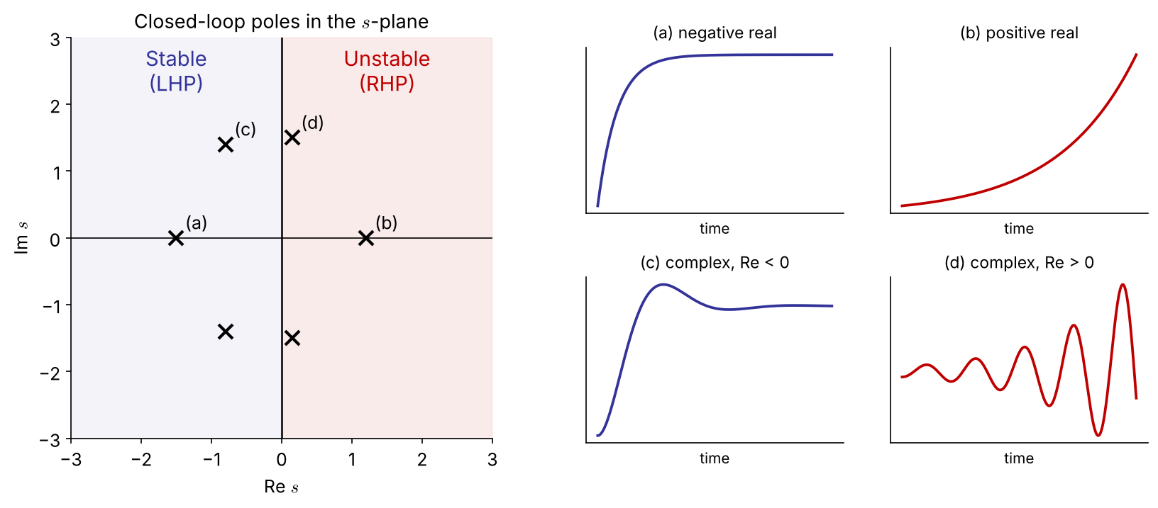
General stability criterion. The closed-loop system is stable if and only if all roots of the characteristic equation lie in the open left-half plane (negative real parts). A root on the imaginary axis → marginally stable; any root in the RHP → unstable.

Pole location ↔︎ time response

Real part → growth/decay rate; imaginary part → oscillation frequency. Stability depends on the sign of the real part only.

Example 4.1   Stabilizing an unstable process with P control

Unstable process \(G_p=\dfrac{K}{s-a}\) \((a>0)\), unity feedback \(G_m=G_a=1\), \(G_c=K_c\):

\[ 1+K_c\frac{K}{s-a}=0 \;\Rightarrow\; s-a+K_cK=0 \;\Rightarrow\; s=a-K_cK \]

Closed loop is stable iff \(\;K_cK>a\)

  • Feedback can create stability, not only lose it (e.g., exothermic CSTR operated at an unstable steady state).
  • There is a minimum gain here; in Ex 4.2 we will meet a maximum gain.

4.2 Routh–Hurwitz Criterion

(1) Hurwitz test: a necessary condition

\[ P(s)=a_ns^n+a_{n-1}s^{n-1}+\cdots+a_1s+a_0,\qquad a_n>0 \]

  • If all roots are in the LHP, then all coefficients are positive (none missing).
  • If any coefficient is negative → at least one root has a positive real part.
  • If any coefficient is zero → not all roots are in the open LHP. FIX
    (The roots may be on the imaginary axis or in the RHP — e.g. \(s^3+1\) has roots \(-1,\ \tfrac12\pm j\tfrac{\sqrt3}{2}\).)

All coefficients positive is necessary but not sufficient for \(n\ge 3\) → we need the Routh array.

(2) Routh array: necessary and sufficient

row
\(s^n\) \(a_n\) \(a_{n-2}\) \(a_{n-4}\)
\(s^{n-1}\) \(a_{n-1}\) \(a_{n-3}\) \(a_{n-5}\)
\(s^{n-2}\) \(b_1\) \(b_2\) \(\cdots\)
\(s^{n-3}\) \(c_1\) \(c_2\) \(\cdots\)
\(\vdots\)
\(s^0\) \(\ast\)

\[ b_1=\frac{a_{n-1}a_{n-2}-a_na_{n-3}}{a_{n-1}},\qquad b_2=\frac{a_{n-1}a_{n-4}-a_na_{n-5}}{a_{n-1}} \] \[ c_1=\frac{b_1a_{n-3}-a_{n-1}b_2}{b_1},\ \ldots \]

Routh criterion. All roots in the LHP ⇔ every element of the first column is positive. FIX

The number of sign changes in the first column = number of RHP roots.

Results worth memorizing

  • \(n=2\): all \(a_i>0\) (that’s all)
  • \(n=3\): all \(a_i>0\) and \(\;a_2a_1>a_3a_0\)

General 4th-order formulas → Appendix

(3) Special cases NEW

Case 1 — zero in the first column

Replace the 0 by a small \(\varepsilon>0\), continue, then let \(\varepsilon\to0^+\).

\(P(s)=s^4+s^3+2s^2+2s+3\)

\(s^4\) 1 2 3
\(s^3\) 1 2
\(s^2\) \(0\to\varepsilon\) 3
\(s^1\) \(2-3/\varepsilon\to-\infty\)
\(s^0\) 3

Two sign changes → 2 RHP roots (\(0.41\pm1.29j\))

Case 2 — a whole row of zeros

The roots contain pairs symmetric about the origin (typically \(\pm j\omega\)).

  1. Form the auxiliary polynomial \(A(s)\) from the row above.
  2. Replace the zero row by \(dA/ds\) and continue.
  3. Roots of \(A(s)=0\) are those symmetric roots.

In stability problems a zero row appears exactly at the ultimate gain, and \(A(j\omega)=0\) gives \(\omega_u\) — see Ex 4.2 at \(K_c=60\).

Example 4.2   P control of a third-order process

\[ 1+K_c\frac{1}{(s+3)(s+2)(s+1)}=0\;\Rightarrow\; s^3+6s^2+11s+(6+K_c)=0 \]

\(s^3\) 1 11
\(s^2\) 6 \(6+K_c\)
\(s^1\) \(\dfrac{66-(6+K_c)}{6}=10-\dfrac{K_c}{6}\) 0
\(s^0\) \(6+K_c\)

First column positive:

  • \(10-K_c/6>0 \Rightarrow K_c<60\)
  • \(6+K_c>0 \Rightarrow K_c>-6\)

\(-6<K_c<60\quad\) (with a positive controller gain: \(0<K_c<60\))

Same as the 3rd-order rule \(a_2a_1>a_3a_0\): \(\;6\cdot11>6+K_c\).

Example 4.2 at \(K_c=60\): a row of zeros NEW

\(s^3\) 1 11
\(s^2\) 6 66
\(s^1\) 0

Auxiliary polynomial from the \(s^2\) row:

\[ A(s)=6s^2+66=0\;\Rightarrow\; s=\pm j\sqrt{11} \]

At the stability limit the closed loop has a pair of pure imaginary poles \(s=\pm j\omega_u\), \(\ \omega_u=\sqrt{11}\) — the system oscillates with constant amplitude.

→ This is exactly what direct substitution (\(s=j\omega\)) looks for (§4.3).

Example 4.3   PI control of a critically damped process

\(G_p=\dfrac{1}{s^2+2s+1}\), \(\;G_c=K_c\left(1+\dfrac{1}{\tau_Is}\right)\):

\[ 1+K_c\frac{\tau_Is+1}{\tau_Is(s^2+2s+1)}=0\;\Rightarrow\; \tau_Is^3+2\tau_Is^2+\tau_I(1+K_c)s+K_c=0 \]

\(s^3\) \(\tau_I\) \(\tau_I(1+K_c)\)
\(s^2\) \(2\tau_I\) \(K_c\)
\(s^1\) \(\tau_I(1+K_c)-\dfrac{K_c}{2}\)
\(s^0\) \(K_c\)

\(K_c>0,\ \tau_I>0,\quad \tau_I>\dfrac{K_c}{2(1+K_c)}\)

  • Since \(\dfrac{K_c}{2(1+K_c)}<\dfrac12\), any \(\tau_I\ge 0.5\) is stable for all \(K_c>0\).
  • Too much integral action (small \(\tau_I\)) is destabilizing.

Routh array in code

import sympy as sp
from routh import routh_array          # routh.py (handles epsilon & zero-row cases)

s, Kc, tI = sp.symbols('s K_c tau_I', positive=True)

R = routh_array((s+3)*(s+2)*(s+1) + Kc, s)                 # Ex 4.2
sp.solve([r[0] > 0 for r in R], Kc)                        # -> Kc < 60

R = routh_array(tI*s*(s**2 + 2*s + 1) + Kc*(tI*s + 1), s)  # Ex 4.3
sp.simplify(R[2][0])                                       # -> tau_I*(Kc+1) - Kc/2

routh_array((s+3)*(s+2)*(s+1) + 60, s)                     # zero row -> A(s) = 6(s^2+11)
syms s Kc tI positive
p = sym2poly_sym(expand((s+3)*(s+2)*(s+1) + Kc), s);   % [1 6 11 Kc+6]
R = routh_array(p);   R(:,1)                         % first column

function c = sym2poly_sym(P, s), c = coeffs(P, s, 'All'); end

function R = routh_array(p)            % basic version (no special cases)
  n = numel(p)-1;  cols = floor(n/2)+1;  R = sym(zeros(n+1, cols));
  R(1,1:numel(p(1:2:end))) = p(1:2:end);
  R(2,1:numel(p(2:2:end))) = p(2:2:end);
  for i = 3:n+1
    for j = 1:cols-1
      R(i,j) = simplify((R(i-1,1)*R(i-2,j+1) - R(i-2,1)*R(i-1,j+1))/R(i-1,1));
    end
  end
end

4.3 Direct-Substitution Analysis

Finding the stability boundary with \(s=j\omega\)

At the moment a system becomes unstable, a pair of closed-loop poles sits on the imaginary axis. Substitute \(s=j\omega\) and set real and imaginary parts to zero:

  • the gain at this limit → ultimate (critical) gain \(K_{cu}\)
  • the frequency → ultimate (crossover) frequency \(\omega_u\), ultimate period \(P_u=2\pi/\omega_u\)

Example 4.2A   \((j\omega)^3+6(j\omega)^2+11(j\omega)+6+K_c=0\)

\[ \text{Im: } \omega(11-\omega^2)=0\Rightarrow \omega_u=\sqrt{11}=3.32,\qquad \text{Re: } 6+K_c-6\omega^2=0\Rightarrow K_{cu}=60 \]

Example 4.3A   With \(s=j\omega\) in \(\tau_Is^3+2\tau_Is^2+\tau_I(1+K_c)s+K_c=0\): Im gives \(\omega_u^2=1+K_c\), Re gives \(K_c=2\tau_I\omega_u^2\) ⇒ \(\tau_I=\dfrac{K_c}{2(1+K_c)}\) — the same boundary as Routh. Direct substitution finds the boundary; Routh gives the region.

Example 4.4   First-order process with dead time

\[ 1+K_c\frac{0.8e^{-2s}}{5s+1}=0 \]

\(e^{-2s}\) is not a polynomial → Routh cannot be applied directly. With \(s=j\omega\):

\[ 0.8K_c\,e^{-2j\omega}=-(1+5j\omega) \]

Magnitude: \(\;0.8K_c=\sqrt{1+25\omega^2}\)

Phase: \(\;-2\omega-\tan^{-1}(5\omega)=-\pi\)

Solve the phase equation numerically:

\(\omega_u=0.895\ \text{rad/time}\)

\(K_{cu}=\dfrac{\sqrt{1+25\omega_u^2}}{0.8}=5.73\)

Stable for \(0<K_c<5.73\).

Dead time: exact vs. Padé approximation NEW

First-order Padé: \(\;e^{-\theta s}\approx\dfrac{1-\theta s/2}{1+\theta s/2}=\dfrac{1-s}{1+s}\;\) ⇒ \(\;5s^2+(6-0.8K_c)s+(1+0.8K_c)=0\) ⇒ \(K_{cu}=7.5\), \(\omega_u=1.18\)
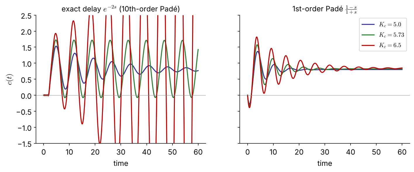
The 1st-order Padé model overestimates the ultimate gain by 31 % (7.5 vs 5.73): at \(K_c=6.5\) it predicts a stable loop that actually oscillates with growing amplitude. Use approximations with care — they err on the unsafe side here.

Dead time in code

import numpy as np, control as ct
from scipy.optimize import brentq

# exact: phase condition -2w - atan(5w) = -pi
wu  = brentq(lambda w: 2*w + np.arctan(5*w) - np.pi, 0.1, 2.0)
Kcu = np.sqrt(1 + 25*wu**2)/0.8                     # 0.895, 5.73

# Pade approximations of e^{-2s}
G = ct.tf(0.8, [5, 1])
for order in (1, 10):
    D = ct.tf(*ct.pade(2, order))
    gm, pm, wcg, wcp = ct.margin(G*D)               # gain margin = Kcu
    print(order, gm, wcg)                           # 1: 7.50, 1.18   10: 5.73, 0.895
wu  = fzero(@(w) 2*w + atan(5*w) - pi, [0.1 2]);
Kcu = sqrt(1 + 25*wu^2)/0.8                % 5.73

G = tf(0.8, [5 1]);
[n1,d1] = pade(2,1);   [Gm1,~,Wcg1] = margin(G*tf(n1,d1))     % 7.50, 1.18
Gd = tf(0.8, [5 1], 'InputDelay', 2);
[Gm, ~, Wcg] = margin(Gd)                                     % exact: 5.73, 0.895

Which technique? (decision chart)

Yes No No Yes Yes No Nonlinear process model Linearize? Transfer- function model Dead time? Routh array Root locus Nonlinear tests (Lyapunov, Khalil 2001) Padé approx.? Direct substitution s = jω or frequency response (Ch. 5) Ex 4.2, 4.3 Ex 4.2B, 4.3B, 4.6–4.8 Ex 4.2A, 4.3A, 4.4 Ex 4.4 (Padé, with error) pole locations → dynamics & design

From \(K_{cu}, P_u\) to controller tuning NEW

The ultimate gain and period are the basis of closed-loop (Ziegler–Nichols) tuning — the starting point for the PID term project.

Controller \(K_c\) \(\tau_I\) \(\tau_D\)
P \(0.5K_{cu}\) — —
PI \(0.45K_{cu}\) \(P_u/1.2\) —
PID \(0.6K_{cu}\) \(P_u/2\) \(P_u/8\)
\(K_{cu}\) \(P_u\) ZN-PI \((K_c,\tau_I)\)
Ex 4.2 60 1.89 27, 1.58
Ex 4.4 5.73 7.02 2.58, 5.85
  • In the plant, \(K_{cu}\) and \(P_u\) are found experimentally (gain ramp-up, or a relay test) — no model needed.
  • ZN settings give a quarter-decay response: a starting point, usually detuned afterwards (tuning rules: Ch 3).

4.4 Root-Locus Analysis

What is a root locus?

Root locus: the paths traced by the closed-loop poles as a parameter (usually \(K_c\)) varies from 0 to \(\infty\).

\[ 1+K_cG_0(s)=0,\qquad G_0=\frac{Q(s)}{P(s)}=\frac{(s-z_1)\cdots(s-z_m)}{(s-p_1)\cdots(s-p_n)} \]

\(K_cG_0\) is the open-loop transfer function (\(G_0=G_mG_aG_p\) for P control; other controllers contribute to \(G_0\)).

\[ (s-p_1)\cdots(s-p_n)+K_c(s-z_1)\cdots(s-z_m)=0 \]

  • \(n\) loci (order of the characteristic polynomial)
  • \(K_c=0\): loci start at the open-loop poles; \(K_c\to\infty\): they end at the open-loop zeros
  • Proper systems \(n\ge m\): the remaining \((n-m)\) loci go to infinity along asymptotes

Angle and magnitude conditions NEW

A point \(s\) is on the locus iff \(K_cG_0(s)=-1\) for some \(K_c>0\):

Angle condition (shapes the locus, independent of \(K_c\)) \[ \sum_j\angle(s-z_j)-\sum_i\angle(s-p_i)=(2k+1)\pi \]

Magnitude condition (gives \(K_c\) at that point) \[ K_c=\frac{\prod_i|s-p_i|}{\prod_j|s-z_j|} \]

Check on Ex 4.2 at \(s=j\sqrt{11}\):

  • angles: \(\tan^{-1}\!\sqrt{11}+\tan^{-1}\!\tfrac{\sqrt{11}}{2}+\tan^{-1}\!\tfrac{\sqrt{11}}{3}=73.2^\circ+58.9^\circ+47.9^\circ=180^\circ\) ✓
  • gain: \(K_c=|j\sqrt{11}+1|\,|j\sqrt{11}+2|\,|j\sqrt{11}+3|=\sqrt{12}\sqrt{15}\sqrt{20}=60\) ✓

Every sketching rule on the next slides follows from these two conditions — and the magnitude condition replaces graphical rlocfind with an exact number.

Sketching rules (1)–(5)

  1. Mark open-loop poles × and zeros ○. The plot is symmetric about the real axis.
  2. Number of loci = number of open-loop poles \(n\).
  3. Loci start at poles (\(K_c=0\)) and end at zeros or at infinity. A \(q\)-th order pole (zero) emits (absorbs) \(q\) loci.
  4. Real axis: a point is on the locus iff the number of real poles + zeros to its right is odd (count multiplicities).
  5. Imaginary-axis crossings: by Routh (zero row) or by \(s=j\omega\).

Sketching rules (6)–(8)

  1. Asymptotes of the \((n-m)\) loci going to infinity: \[ \gamma=\frac{\sum p_i-\sum z_j}{n-m},\qquad \theta_k=\frac{(2k+1)\pi}{n-m},\ k=0,\ldots,n-m-1 \]
  2. Departure / arrival angles at complex poles / zeros (\(q\) = multiplicity): \[ q\phi_{\text{dep}}=\sum\psi_j-\sum_{\text{other}}\phi_i-(2k+1)\pi,\qquad q\psi_{\text{arr}}=\sum\phi_i-\sum_{\text{other}}\psi_j+(2k+1)\pi \]
  3. Break-away / break-in points (multiple roots) on the real axis: \[ Q(s)\frac{dP}{ds}-P(s)\frac{dQ}{ds}=0 \] Two branches meet at 180° and leave at ±90°; three meet at 120° and leave rotated by 60°.

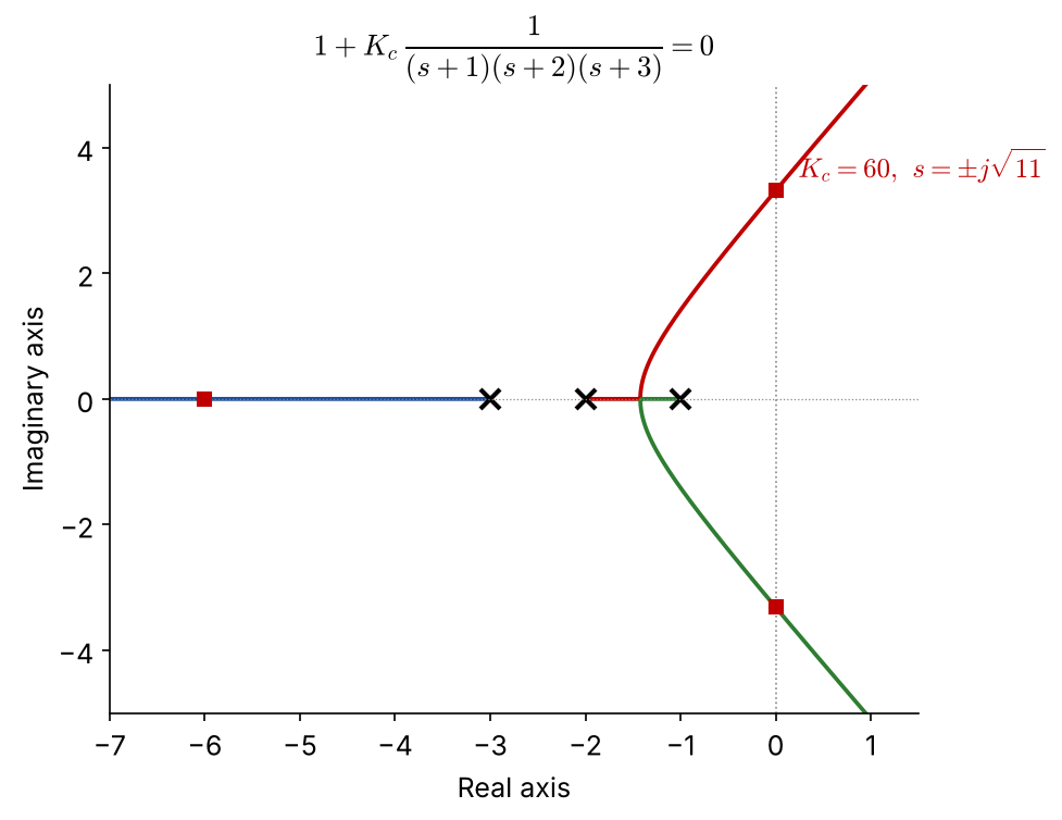
Example 4.2B   Root locus of Ex 4.2

  • Poles \(-1,-2,-3\); no zeros; \(n-m=3\)
  • Real axis: \((-2,-1)\) and \((-\infty,-3)\)
  • Asymptotes: \(\gamma=\dfrac{-6}{3}=-2\), \(\ \theta=\pm60^\circ,180^\circ\)
  • Break-away: \(\dfrac{dP}{ds}=3s^2+12s+11=0\) \(\Rightarrow s=-1.42\) (the other root \(-2.58\) is not on the locus)
  • Crossing: \(s=\pm j\sqrt{11}\) at \(K_{cu}=60\) (Routh / direct substitution)

Three methods, one answer: \(K_{cu}=60,\ \omega_u=\sqrt{11}\)

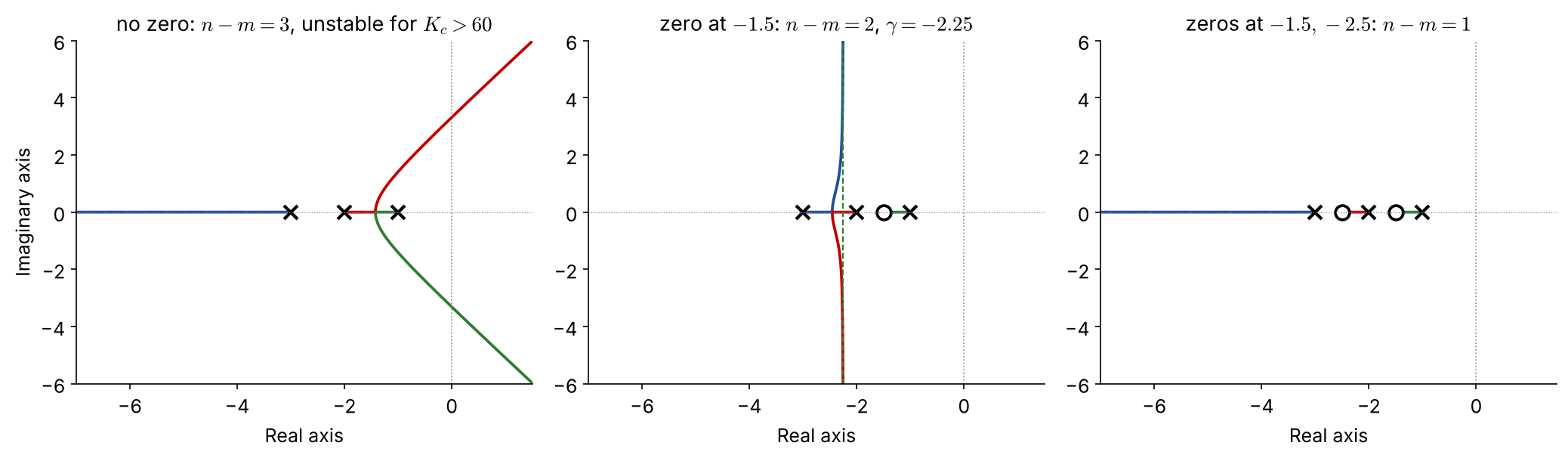
Example 4.6   Representative root-locus shapes
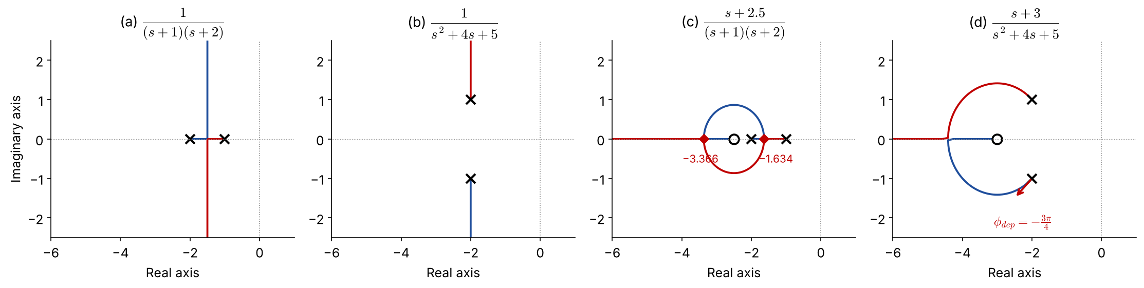
  1. real poles: break-away at \(-1.5\), vertical asymptotes; always stable
  1. complex poles: vertical lines from \(-2\pm j\); always stable, more oscillatory
  1. zero at \(-2.5\): loci leave the axis and return — a circle around the zero
  1. complex poles + zero: departure angle \(\mp3\pi/4\), break-in at \(-4.41\)

Example 4.6 (c), (d): the calculations

(c) \(\;G_0=\dfrac{s+2.5}{(s+1)(s+2)}\), \(\;P=s^2+3s+2\), \(\;Q=s+2.5\)

\[ \begin{aligned} Q\frac{dP}{ds}-P\frac{dQ}{ds}&=(s+2.5)(2s+3)\\ &\quad-(s^2+3s+2)\\ &=s^2+5s+5.5=0 \end{aligned} \]

\(s=-1.634\) (break-away), \(\ s=-3.366\) (break-in)

(d) \(\;G_0=\dfrac{s+3}{s^2+4s+5}\), poles \(-2\pm j\), zero \(-3\)

Departure from the lower pole \(p_2=-2-j\): FIX

  • from zero \(-3\): \(\ \psi=\angle(1-j)=-\pi/4\)
  • from pole \(p_1=-2+j\): \(\ \phi_1=\angle(-2j)=-\pi/2\)

\[ \phi_{\text{dep}}=-\tfrac{\pi}{4}-\left(-\tfrac{\pi}{2}\right)-\pi=-\tfrac{3\pi}{4} \] (upper pole: \(+3\pi/4\) by symmetry)

Effect of adding a zero NEW

  • One LHP zero reduces \(n-m\) from 3 to 2: asymptotes become vertical at \(\gamma=\dfrac{-6-(-z)}{2}<0\) → loci never cross into the RHP
  • Holds for any zero \(z\in\{0.5,1.5,2.5,3.5\}\): \(\gamma=-2.75\ldots-1.25\)

An LHP zero pulls the loci to the left (stabilizing). A PD controller \(K_c(1+\tau_Ds)\) adds exactly such a zero → Problem #1.

Effect of adding a pole: PI control (Example 4.3B)
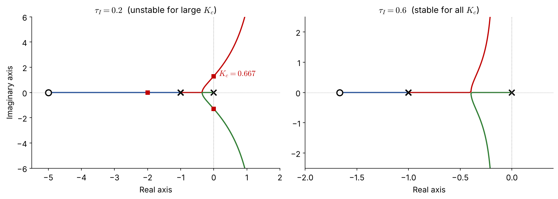
PI adds a pole at the origin and a zero at \(-1/\tau_I\); \(n-m=2\), \(\ \gamma=\dfrac{-2+1/\tau_I}{2}\)

  • \(\tau_I=0.2\): \(\gamma=+1.5\) → crosses at \(K_c=0.667\) (Routh: \(\tau_I=\frac{K_c}{2(1+K_c)}\) ✓)
  • \(\tau_I=0.6\): \(\gamma=-0.17\) → stable for all \(K_c\)

Adding poles pushes loci to the right (destabilizing). Keep the PI zero far enough left (\(\tau_I>0.5\) here).

RHP zero: inverse response NEW
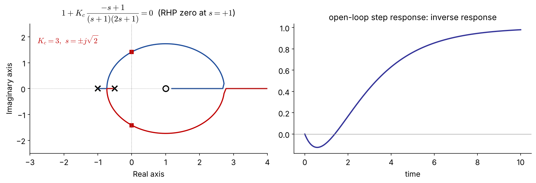
\(1+K_c\dfrac{-s+1}{(s+1)(2s+1)}=0 \Rightarrow 2s^2+(3-K_c)s+(1+K_c)=0\) → stable only for \(0<K_c<3\).

A locus ends at the RHP zero \(s=+1\), so high gain is always unstable — no controller tuning can remove this limit. Typical of inverse-response processes (e.g. drum-level “swell”, some reactors).

4.5 Root-Locus Design

Dominant poles and performance specs

Approximate the closed loop by its dominant underdamped pair

\[ s=-\frac{\zeta}{\tau}\pm j\frac{\sqrt{1-\zeta^2}}{\tau},\quad |s|=\frac1\tau=\omega_n,\quad \zeta=\cos\psi \]

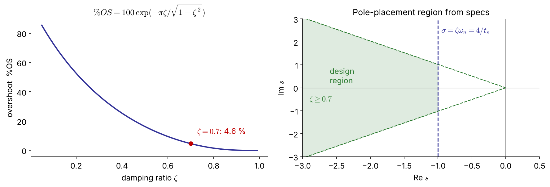
NEW \(\;\%OS=100\exp\!\left(-\dfrac{\pi\zeta}{\sqrt{1-\zeta^2}}\right),\qquad t_s(2\%)\approx\dfrac{4}{\zeta\omega_n}\)

\(\zeta\) spec → a ray at angle \(\psi\); \(\ t_s\) spec → a vertical line \(\mathrm{Re}\,s=-4/t_s\)
Example 4.7   Gain for \(\zeta=0.7\) (P control)

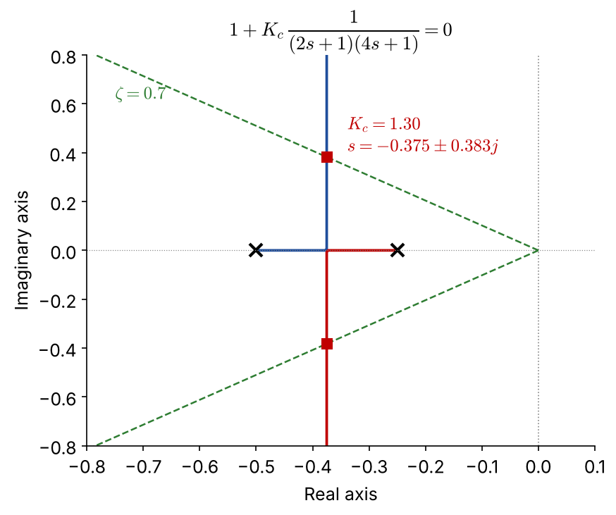
\(G_p=\dfrac{1}{(2s+1)(4s+1)}\) \(\;(K_p=1,\ \tau_1=2,\ \tau_2=4)\): \(\;8s^2+6s+(1+K_c)=0\)

\[ \omega_n^2=\frac{1+K_c}{8},\quad 2\zeta\omega_n=\frac{6}{8} \;\Rightarrow\;\zeta=\frac{3}{\sqrt{8(1+K_c)}} \]

\(\zeta=0.7\ \Rightarrow\ K_c=\dfrac{127}{98}=1.30\) FIX

poles \(-0.375\pm0.383j\), \(\ \%OS=4.6\%\), \(\ t_s\approx11\)

  • Graphical rlocfind gave 1.23 — use the magnitude condition for an exact value.
  • Offset: \(\dfrac{1}{1+K_c}=0.44\) (!) → P control alone is not enough → Ex 4.8 (PI)
Example 4.7 in code

import numpy as np, control as ct, matplotlib.pyplot as plt

G = ct.tf(1, np.polymul([2, 1], [4, 1]))
ct.root_locus_plot(G, grid=True)                 # s-plane grid incl. zeta lines
zeta = 0.7
# analytic: zeta = 3/sqrt(8(1+Kc))
Kc = 9/(8*zeta**2) - 1                           # 1.296
print(Kc, ct.feedback(Kc*G, 1).poles())          # -0.375 ± 0.383j
print(ct.step_info(ct.feedback(Kc*G, 1)))        # overshoot 4.6 %
G = tf(1, conv([2 1],[4 1]));
rlocus(G); axis([-0.8 0 -1 1]); sgrid(0.7, 0.2:0.2:1)   % wn > 0
zeta = 0.7;
Kc = 9/(8*zeta^2) - 1                 % exact: 1.296  (rlocfind click: ~1.23)
pole(feedback(Kc*G,1))
stepinfo(feedback(Kc*G,1))

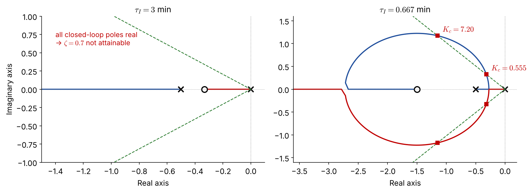
Example 4.8   PI design for \(\zeta=0.7\)

First-order process \(K_p=0.5\), \(\tau_p=2\) min, \(G_a=G_m=1\):

\[ 1+K_c\frac{0.5(\tau_Is+1)}{\tau_Is(2s+1)}=0\;\Rightarrow\; 2\tau_Is^2+\tau_I(1+0.5K_c)s+0.5K_c=0 \]

(a) \(\tau_I=3\) min: zero at \(-1/3\) lies between the poles \(0\) and \(-1/2\)

\(\zeta=\dfrac{3(1+0.5K_c)}{2\sqrt{3K_c}}\ \ge\ 1.22\) for all \(K_c\)

→ always overdamped; \(\zeta=0.7\) is not attainable

(b) \(\tau_I=2/3\) min: zero at \(-1.5\) — loci form a circle

\(\zeta=0.7\Rightarrow 0.0625K_c^2-0.485K_c+0.25=0\)

\(K_c=0.555\) FIX: poles \(-0.32\pm0.33j\), \(t_s\approx12\) min

\(K_c=7.20\) FIX: poles \(-1.15\pm1.17j\), \(t_s\approx3\) min

Example 4.8: root loci and a caveat

  • Choose \(K_c=7.20\) for the faster response.
  • Caveat: the PI zero at \(-1.5\) is close to the dominant poles → actual overshoot is 13 %, not 4.6 %. The second-order approximation must be checked by simulation.
  • Alternative: \(\tau_I=\tau_p=2\) cancels the process pole → \(1+\dfrac{0.5K_c}{2s}=0\), a first-order closed loop with \(\tau_{cl}=4/K_c\).

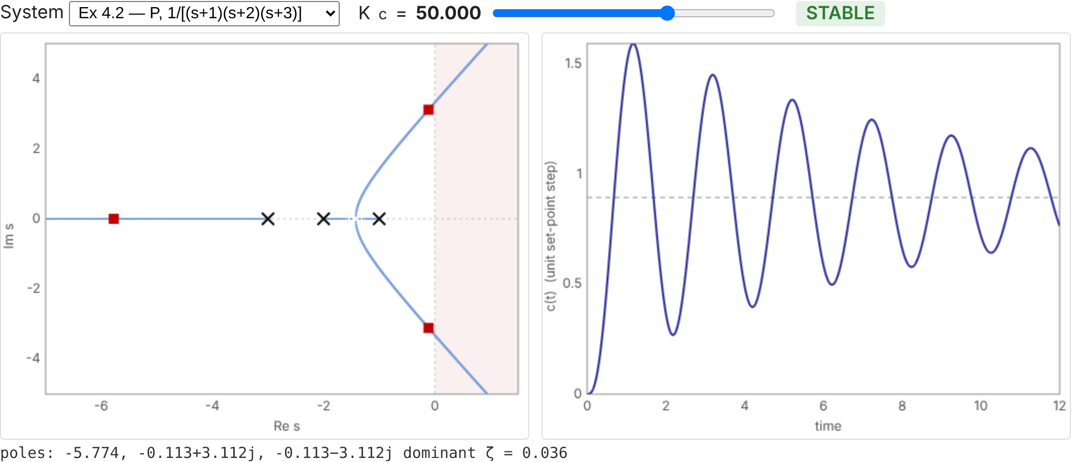
Interactive: move \(K_c\), watch poles and response NEW
Final remarks on root-locus plots

  1. Root locus cannot handle dead time easily — frequency-response analysis handles it exactly (Ch. 5).
  2. Root locus gives absolute stability only; there is no general “safety margin” — frequency response defines relative stability (gain/phase margins).
  3. In return, root locus shows the dynamic response (damping, speed) directly — something frequency response does not do easily.

Toolbox summary

Task MATLAB Python (control, scipy, sympy)
transfer function tf(num,den) ct.tf(num,den)
root locus rlocus(G), sgrid ct.root_locus_plot(G, grid=True)
closed loop / poles feedback, pole ct.feedback, .poles()
Padé / margins pade, margin ct.pade, ct.margin
Routh array (custom function) routh.py (sympy)
step response step, stepinfo ct.step_response, ct.step_info

Problem #1   (homework)

\[ G_p=\frac{2(s+1)}{s(s+2)(s^2+1)},\qquad 1+G_cG_p=0 \]

  1. Show with an analytical technique of your choice that the closed loop cannot be stabilized by a proportional controller.

  2. With a PI or a PD controller (positive gain), write the characteristic equations. Without further analysis, which is more likely to stabilize the system?

  3. Use root-locus plots to illustrate your answer.

Resources

Appendix

Routh array: 4th-order polynomial

\(p(s)=a_4s^4+a_3s^3+a_2s^2+a_1s+a_0\)

\(s^4\) \(a_4\) \(a_2\) \(a_0\)
\(s^3\) \(a_3\) \(a_1\) 0
\(s^2\) \(b_1=\dfrac{a_3a_2-a_4a_1}{a_3}\) \(b_2=a_0\)
\(s^1\) \(c_1=\dfrac{b_1a_1-a_3a_0}{b_1}\) 0
\(s^0\) \(d_1=a_0\)

Stable ⇔ all \(a_i>0\), \(\;b_1>0\), \(\;c_1>0\), i.e. \(\;a_3a_2>a_4a_1\;\) and \(\;a_3a_2a_1>a_4a_1^2+a_3^2a_0\).