Process Dynamics and Control

5. Frequency-Response Analysis & Design

Kee-Youn Yoo

Department of Chemical & Biomolecular Engineering, SeoulTech

What are we up to?

Frequency-response analysis is the substitution \(s=j\omega\): everything we need is the magnitude \(|G(j\omega)|\) and the phase \(\angle G(j\omega)\).

  • Impose a sinusoidal input and measure the response — dynamics can be identified even without a model
  • Bode and Nyquist plots are two pictures of the same functions of \(\omega\)
  • Gives a relative stability measure (gain and phase margins) and handles dead time exactly

Running examples

  • Ex 5.10–5.13: inverse-response process \(\dfrac{3(-2s+1)}{(10s+1)(5s+1)}\) under P and PI control
  • Ex 4.4 revisited: \(\dfrac{0.8e^{-2s}}{5s+1}\) — the dead-time case Routh could not do exactly

5.1 Magnitude and Phase Lag

A sine in, a sine out

First-order process \(\;\tau_p\dfrac{dy}{dt}+y=K_pu,\quad G(s)=\dfrac{K_p}{\tau_ps+1},\quad u=A\sin\omega t\):

\[ y(t)=\underbrace{\frac{AK_p\tau_p\omega}{\tau_p^2\omega^2+1}e^{-t/\tau_p}}_{\to\,0} +\frac{AK_p}{\sqrt{\tau_p^2\omega^2+1}}\sin(\omega t+\phi),\qquad \phi=-\tan^{-1}(\omega\tau_p) \]
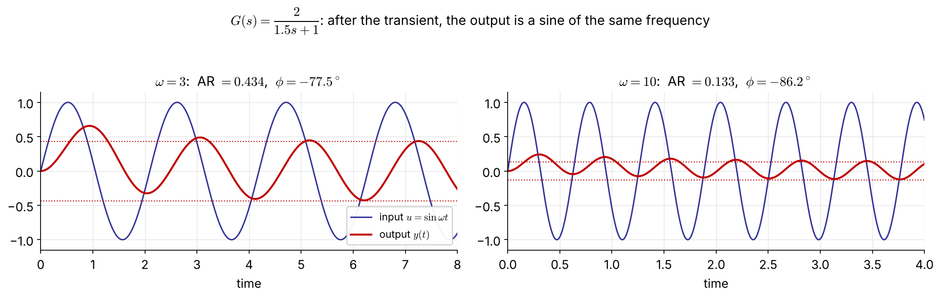
Same frequency; the amplitude ratio \(\text{AR}=K_p/\sqrt{\tau_p^2\omega^2+1}\) falls and the phase lag grows as \(\omega\) increases.

… and \(G(j\omega)\) gives AR and \(\phi\) directly

\[ G(j\omega)=\frac{K_p}{j\omega\tau_p+1}=\frac{K_p}{\tau_p^2\omega^2+1}-j\,\frac{K_p\omega\tau_p}{\tau_p^2\omega^2+1}=|G(j\omega)|\,e^{j\phi} \]

\[ |G(j\omega)|=\frac{K_p}{\sqrt{\tau_p^2\omega^2+1}},\qquad \phi=\angle G(j\omega)=-\tan^{-1}(\omega\tau_p) \]

General result (any stable \(G\), see Appendix for the derivation): at large times

\[ \frac{y_\infty(t)}{A}=|G(j\omega)|\,\sin\big(\omega t+\angle G(j\omega)\big) \]

No partial fractions needed — substitute \(s=j\omega\) and take modulus and argument.

Products of transfer functions

For \(\;G(s)=\dfrac{G_a(s)G_b(s)\cdots G_m(s)}{G_1(s)G_2(s)\cdots G_n(s)}\):

\[ \log|G(j\omega)|=\sum_{\text{num}}\log|G_a(j\omega)|-\sum_{\text{den}}\log|G_i(j\omega)|,\qquad \angle G(j\omega)=\sum_{\text{num}}\angle G_a(j\omega)-\sum_{\text{den}}\angle G_i(j\omega) \]

On log scales, magnitudes add and phases add → a Bode plot is the sum of simple pieces.

Example 5.1   \(G(s)=\dfrac{\tau_as+1}{(\tau_1s+1)(\tau_2s+1)}\) NEW

\[ |G(j\omega)|=\frac{\sqrt{1+\omega^2\tau_a^2}}{\sqrt{1+\omega^2\tau_1^2}\,\sqrt{1+\omega^2\tau_2^2}},\qquad \phi=\tan^{-1}(\omega\tau_a)-\tan^{-1}(\omega\tau_1)-\tan^{-1}(\omega\tau_2) \]

(The original slide left this blank — solution added.)

5.2 Graphical Analysis Tools

Bode and Nyquist plots

Bode plot — two plots against \(\log\omega\)

  • magnitude: log–log (\(|G|\) or dB \(=20\log_{10}|G|\))
  • phase: semi-log, in degrees
  • frequency in rad per unit time

Nyquist (polar) plot — \(G(j\omega)\) drawn in the complex \(G\)-plane with \(\omega\) as the parameter FIX

\[ G(j\omega)=\mathrm{Re}\,G+j\,\mathrm{Im}\,G=|G|e^{j\phi} \]

Same information; more compact, but \(\omega\) is not shown explicitly.

AR dB
0.01 −40
0.1 −20
0.5 −6
1 0
2 +6
10 +20
100 +40

A factor 10 is 20 dB; a factor 2 is ≈ 6 dB.

Example 5.2   First-order lag \(\;K_p/(\tau_ps+1)\)
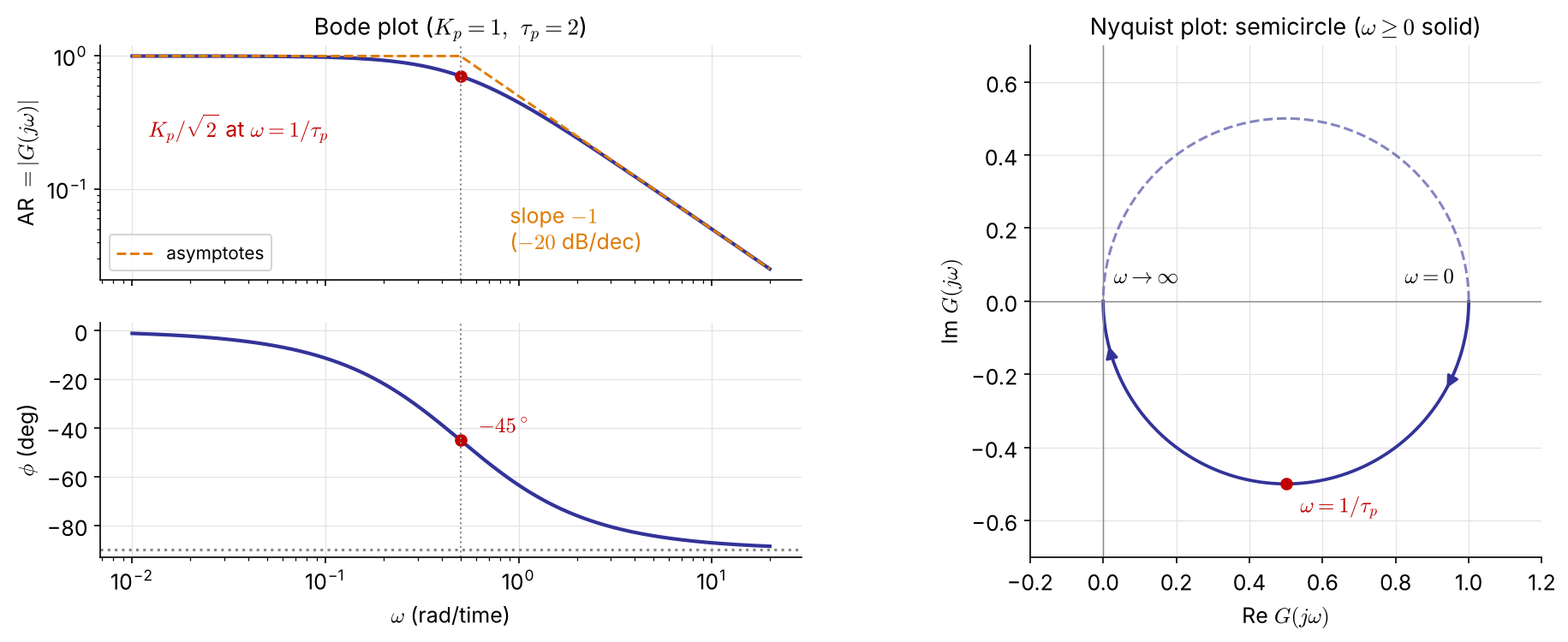
  • \(\omega\to0\): \(|G|=K_p,\ \phi=0\); \(\ \omega\to\infty\): \(|G|\to K_p/\tau_p\omega,\ \phi\to-90^\circ\)
  • Corner frequency \(\omega=1/\tau_p\): \(|G|=K_p/\sqrt2,\ \phi=-45^\circ\)
  • Bandwidth \(\omega_b\): where \(|G|\) drops to 0.707 of its low-frequency value (\(=1/\tau_p\) here)
  • A low-pass filter: small \(\tau\) ⇒ wide bandwidth ⇒ fast system

Example 5.3   Second-order \(\;K/(\tau^2s^2+2\zeta\tau s+1)\)

\[ G(j\omega)=\frac{K\left[(1-\tau^2\omega^2)-j\,2\zeta\tau\omega\right]}{(1-\tau^2\omega^2)^2+(2\zeta\tau\omega)^2} \] \[ |G|=\frac{K}{\sqrt{(1-\tau^2\omega^2)^2+(2\zeta\tau\omega)^2}} \] \[ \phi=\tan^{-1}\!\frac{-2\zeta\tau\omega}{1-\tau^2\omega^2}\quad(0\to-180^\circ) \]

  • \(\omega\to0\): \(\ |G|=K,\ \phi=0\)
  • \(\omega=1/\tau\): \(\ |G|=K/2\zeta,\ \phi=-90^\circ\)
  • \(\omega\to\infty\): \(\ |G|\to K/\tau^2\omega^2\) (slope \(-2\)), \(\ \phi\to-180^\circ\)

Resonance for \(0<\zeta<1/\sqrt2\) FIX \[ \omega_r=\frac{\sqrt{1-2\zeta^2}}{\tau},\qquad M_{p\omega}=\frac{K}{2\zeta\sqrt{1-\zeta^2}} \] Smaller \(\zeta\) → higher peak → more overshoot in time (derivation: Appendix).

The original said the curve rises above \(K\) for \(\zeta<1/2\); that is the condition for \(|G(j/\tau)|>K\). The resonant peak itself exists for \(\zeta<0.707\).

Example 5.3: Bode and Nyquist for \(\zeta=1.2\ldots0.2\)
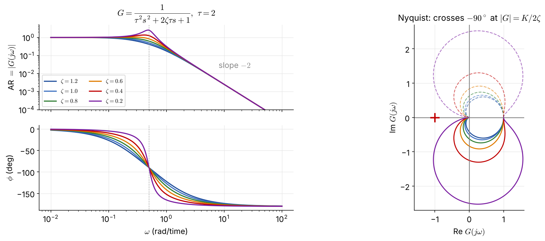
Low damping: a sharp resonant peak in \(|G|\) and a fast phase drop at \(\omega=1/\tau\); the Nyquist curve bulges far beyond the radius-\(K\) circle.

Examples 5.4, 5.7, 5.8: lead, integrator, lag + integrator
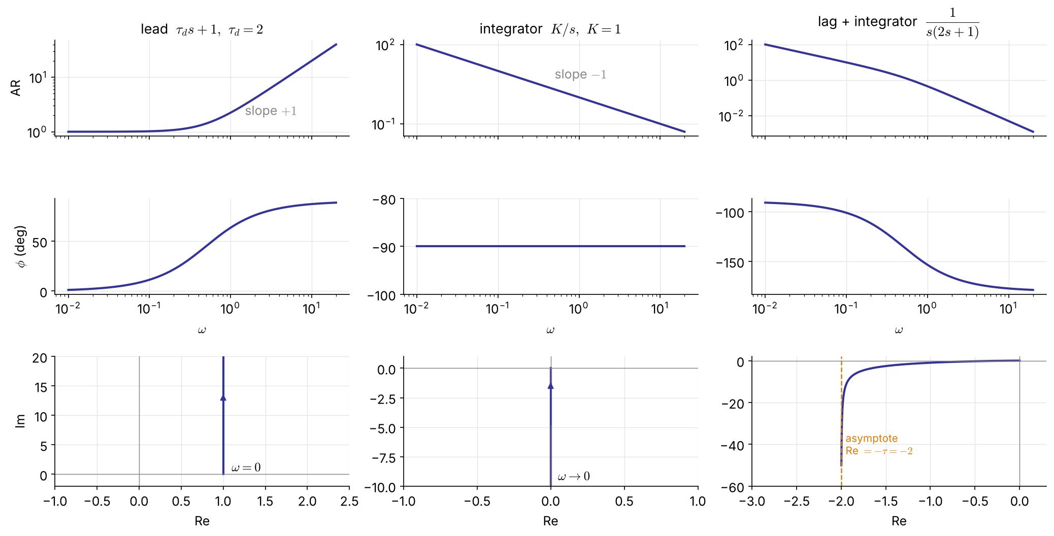
\(|G|=\sqrt{1+\omega^2\tau_d^2}\), \(\ \phi=+\tan^{-1}\omega\tau_d\) (phase lead)

\(|G|=K/\omega\), \(\ \phi=-90^\circ\) for all \(\omega\)

\(\phi\) from \(-90^\circ\) to \(-180^\circ\); Nyquist asymptote \(\mathrm{Re}=-\tau\)

Examples 5.5, 5.6: dead time
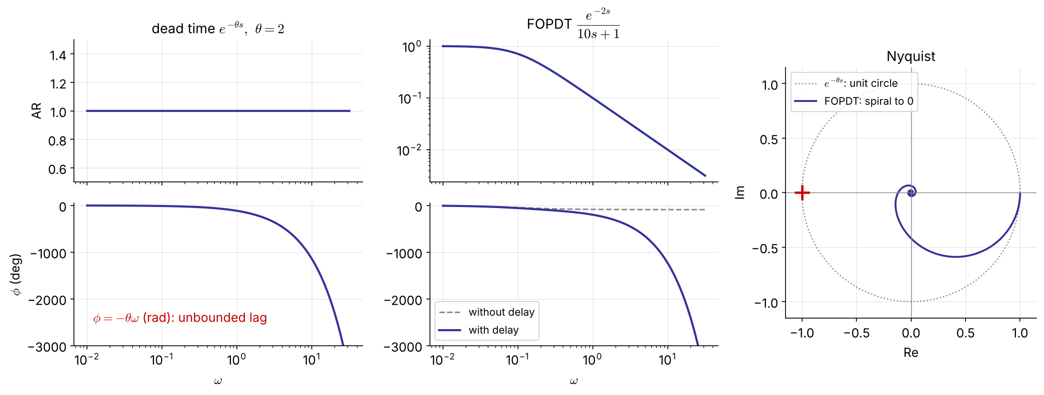
\(|e^{-j\omega\theta}|=1,\ \angle e^{-j\omega\theta}=-\omega\theta\) (rad): the phase lag grows without bound. FOPDT: \(|G|=\dfrac{K_p}{\sqrt{1+\omega^2\tau_p^2}},\ \ \phi=-\tan^{-1}(\omega\tau_p)-\omega\theta\).

Nonminimum-phase systems contain dead time or RHP zeros (Ex 5.10); a minimum-phase system has neither, and no RHP poles.

Building blocks at a glance

Factor AR \(=|G(j\omega)|\) \(\phi=\angle G(j\omega)\) high-\(\omega\) slope \(\phi\) range
\(K\) \(K\) \(0\) \(0\) \(0\)
\(\dfrac{1}{\tau s+1}\) \(\dfrac{1}{\sqrt{1+\omega^2\tau^2}}\) \(-\tan^{-1}\omega\tau\) \(-1\) \(0\to-90^\circ\)
\(\tau s+1\)
(LHP zero)
\(\sqrt{1+\omega^2\tau^2}\) \(+\tan^{-1}\omega\tau\) \(+1\) \(0\to+90^\circ\)
\(-\tau s+1\)
(RHP zero)
\(\sqrt{1+\omega^2\tau^2}\) \(-\tan^{-1}\omega\tau\) \(+1\) \(0\to-90^\circ\)
\(\dfrac{1}{s}\) \(\dfrac1\omega\) \(-90^\circ\) \(-1\) —
\(s\) \(\omega\) \(+90^\circ\) \(+1\) —
\(\dfrac{1}{\tau^2s^2+2\zeta\tau s+1}\) see Ex 5.3 \(-2\) \(0\to-180^\circ\)
\(e^{-\theta s}\) \(1\) \(-\omega\theta\) \(0\) unbounded

Sketching a Bode plot by asymptotes NEW

  1. Write \(G\) in time-constant form \(\;K\dfrac{\prod(\tau_as+1)}{s^q\prod(\tau_is+1)}e^{-\theta s}\) and list the corner frequencies \(1/\tau\).
  2. Low frequency: \(|G|\approx K/\omega^q\) — a line of slope \(-q\) (\(q=0\): horizontal at \(K\)).
  3. Moving right, at each corner the slope changes by −1 for a pole, +1 for a zero (−2 for an underdamped pair).
  4. Phase: each pole contributes \(0\to-90^\circ\) (−45° at its corner), each zero \(0\to+90^\circ\); dead time adds \(-\omega\theta\).

For real poles and zeros the asymptotes are within 3 dB of the exact curve (largest error at a corner; underdamped pairs can deviate more near resonance) — good enough to read crossover frequencies and margins by hand.

Example 5.9   \((5s+1)/[(10s+1)(2s+1)]\) by asymptotes
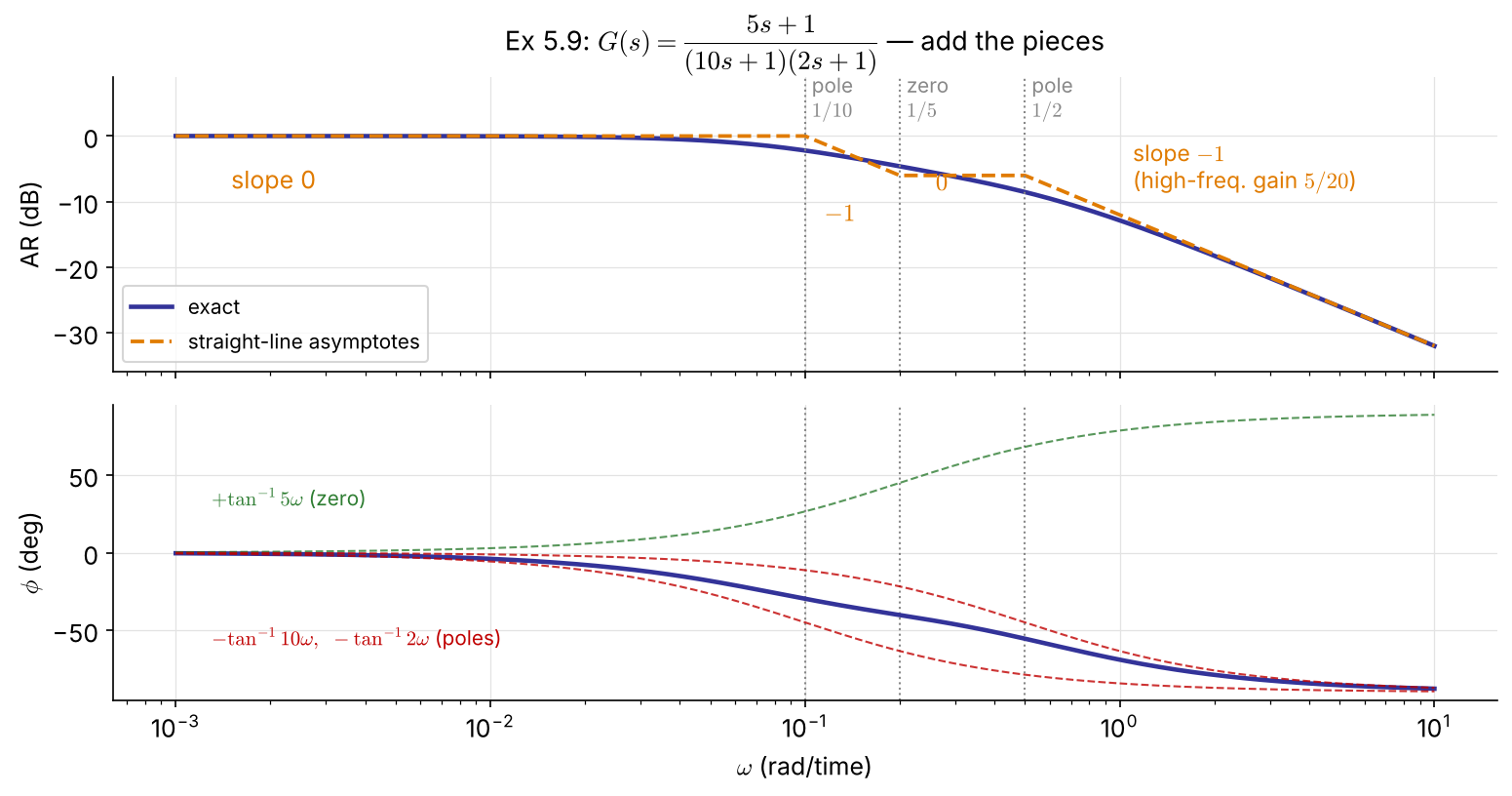
Corners: \(0.1\) (pole), \(0.2\) (zero), \(0.5\) (pole)

\(\omega\) range slope
\(<0.1\) \(0\)
\(0.1\)–\(0.2\) \(-1\)
\(0.2\)–\(0.5\) \(0\)
\(>0.5\) \(-1\)

High frequency: \(|G|\to\dfrac{5}{20\omega}\), \(\ \phi\to-90^\circ\)

Phase: \(\tan^{-1}5\omega-\tan^{-1}10\omega-\tan^{-1}2\omega\) never reaches \(-90^\circ\) at finite \(\omega\)

Bode and Nyquist in code

import numpy as np, control as ct, matplotlib.pyplot as plt

G = ct.tf(1, [2, 1])                              # Ex 5.2
ct.bode_plot(G, dB=False, deg=True)               # AR (log) and phase (deg)
ct.nyquist_plot(G)

# dead time: evaluate G(jw) e^{-jw*theta} exactly (no Pade)
w = np.logspace(-3, 2, 2000)
g = ct.tf(1, [10, 1])(1j*w) * np.exp(-2j*w)       # Ex 5.6, theta = 2
mag, phase = np.abs(g), np.degrees(np.unwrap(np.angle(g)))
fig, (a1, a2) = plt.subplots(2, 1, sharex=True)
a1.loglog(w, mag); a2.semilogx(w, phase)
G = tf(1, [2 1]);                       % Ex 5.2
figure(1), bode(G)
figure(2), nyquist(G)

G6 = tf(1, [10 1], 'InputDelay', 2);    % Ex 5.6: exact dead time
figure(3), bode(G6)
figure(4), nyquist(G6)

K = 1; tau = 2;                         % Ex 5.3: family in zeta
for zeta = [1.2 1.0 0.8 0.6 0.4 0.2]
    bode(tf(K, [tau^2 2*zeta*tau 1])), hold on
end

5.3 Stability Analysis

Two frequency-domain tests

Bode stability criterion

\(G_{OL}\) strictly proper, no poles on or right of the imaginary axis (a single pole at the origin is allowed), and one phase crossover \(\omega_c\) (\(\angle G_{OL}=-180^\circ\)) and one gain crossover \(\omega_g\) (\(|G_{OL}|=1\)):

closed loop stable \(\iff |G_{OL}(j\omega_c)|<1\)

Applies with dead time — unlike Routh.

Nyquist stability criterion

\(G_{OL}\) proper, no unstable pole–zero cancellations.

  • \(N\) = clockwise encirclements of \((-1,0)\) by the Nyquist plot (\(\omega:-\infty\to\infty\))
  • \(P\) = open-loop poles in the RHP
  • \(Z\) = closed-loop poles in the RHP

\[Z=N+P\qquad\text{stable}\iff Z=0\]

FIX (the original had \(Z=N-P\); with clockwise \(N\) the sign is \(+\))

Reading the Nyquist criterion

  • Most process loops are open-loop stable: \(P=0\Rightarrow Z=N\) — unstable iff the curve encircles \(-1\).
  • A counterclockwise encirclement counts \(N=-1\): each one can stabilize one open-loop unstable pole.
  • Nyquist works where Bode does not: open-loop unstable processes, several crossover frequencies.
Yes Yes No No GM, PM = distance of the curve from −1 Open loop GOL(jω) Open-loop stable? One −180° crossing? Bode criterion |GOL(jωc)| < 1 GM, PM → choose Kc Nyquist criterion Z = N + P = 0 (count encirclements of −1) Ex 5.11, Ex 4.4 revisited Ex 5.12, 5.13 Ex 5.14: open-loop unstable process P ≠ 0 several ωc, ωg (a single pole at the origin is allowed in “open-loop stable”)

Examples 5.10, 5.11   Inverse-response process, P control

\(G=\dfrac{3(-2s+1)}{(10s+1)(5s+1)}\) has a RHP zero at \(s=0.5\) → high gain is fundamentally limited.

\[ (10s+1)(5s+1)+3K_c(-2s+1)=0\iff 50s^2+(15-6K_c)s+(1+3K_c)=0 \]

Routh: \(\;15-6K_c>0,\ 1+3K_c>0\;\Rightarrow\;-\tfrac13<K_c<2.5\) \(\quad\) → ultimate gain \(K_u=2.5\); at \(K_u\): \(50s^2+8.5=0\), \(s=\pm j0.412\)
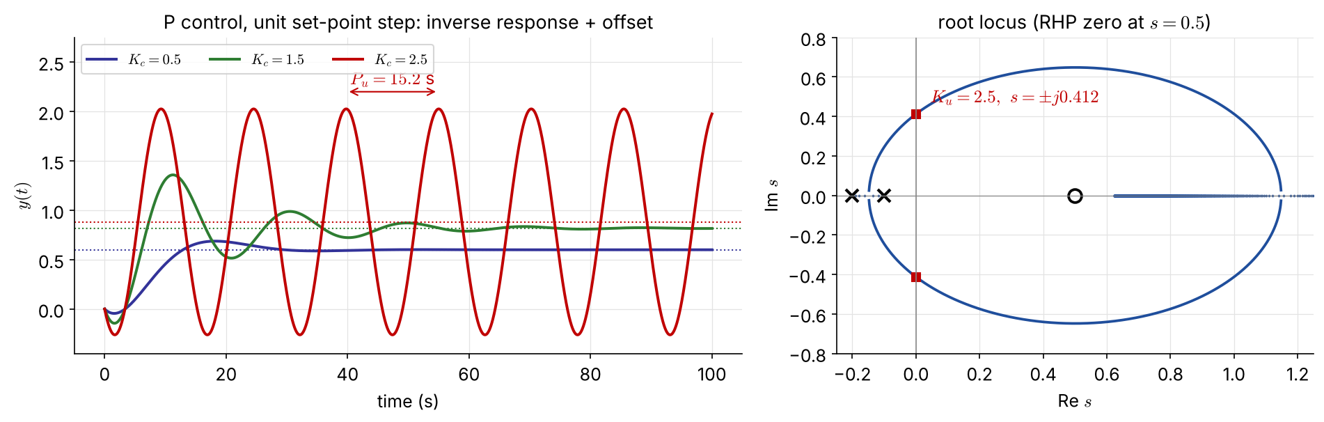
Example 5.11 by frequency response
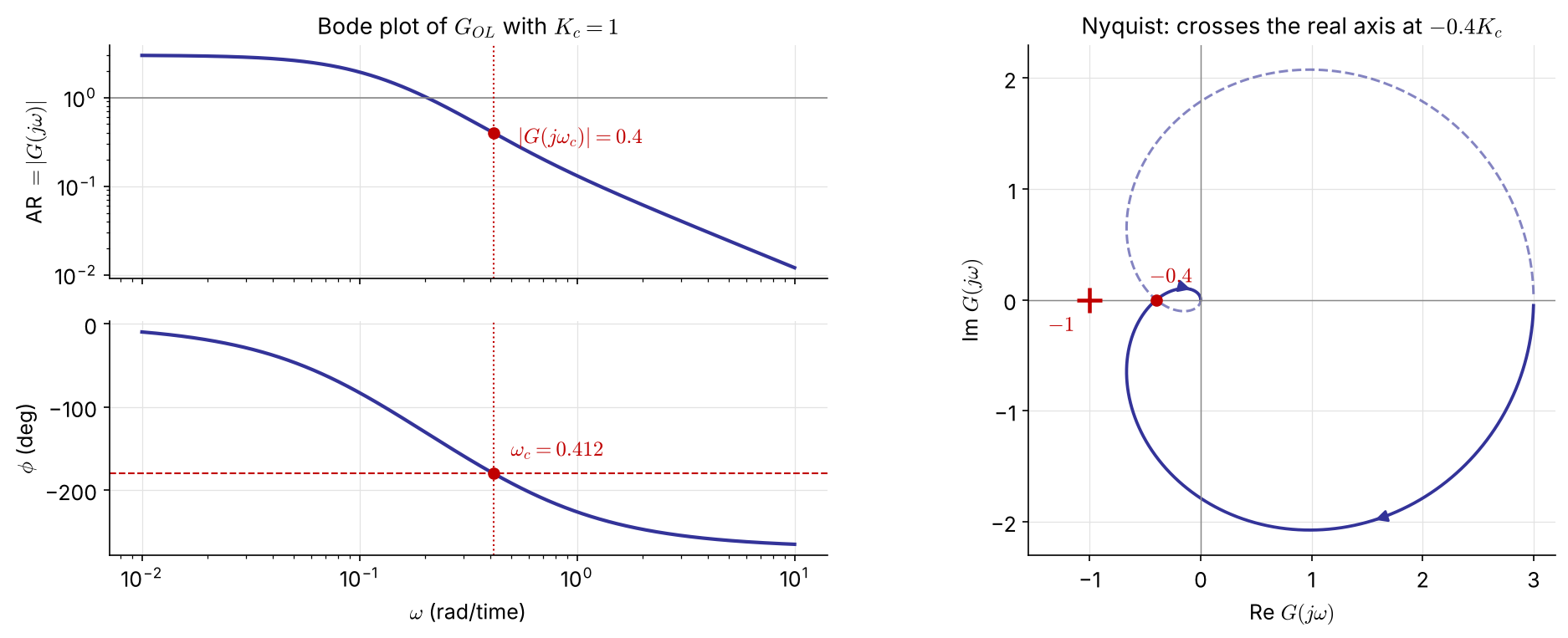
With \(K_c=1\): phase crossover \(\omega_c=0.412\), \(\ |G(j\omega_c)|=0.4\)

\(|G_{OL}(j\omega_c)|=0.4K_c<1\iff\) \(K_c<2.5\) — the same as Routh

Nyquist: the real-axis crossing at \(-0.4K_c\) reaches \(-1\) when \(K_c=2.5\); \(\ P_u=2\pi/\omega_c=15.2\) s

Ex 4.4 revisited: dead time handled exactly NEW
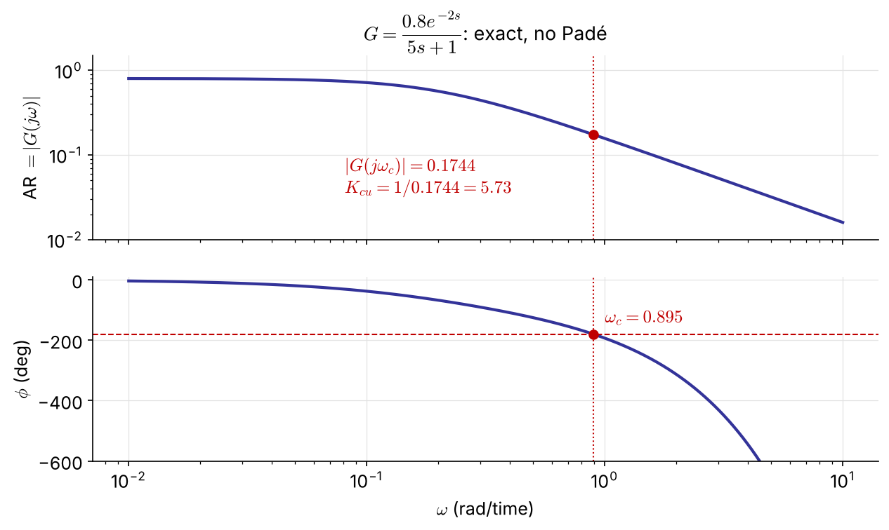
\(G_{OL}=K_c\dfrac{0.8e^{-2s}}{5s+1}\)

Phase crossover: \(\;-\tan^{-1}(5\omega_c)-2\omega_c=-\pi\) \(\Rightarrow\omega_c=0.895\)

\[ K_{cu}=\frac{1}{|G(j\omega_c)|}=\frac{\sqrt{1+25\omega_c^2}}{0.8}=5.73 \]

The same answer as direct substitution in Ch 4 — read off one Bode plot, with no Padé approximation (1st-order Padé gave 7.5).

Example 5.14   Nyquist for an open-loop unstable process NEW
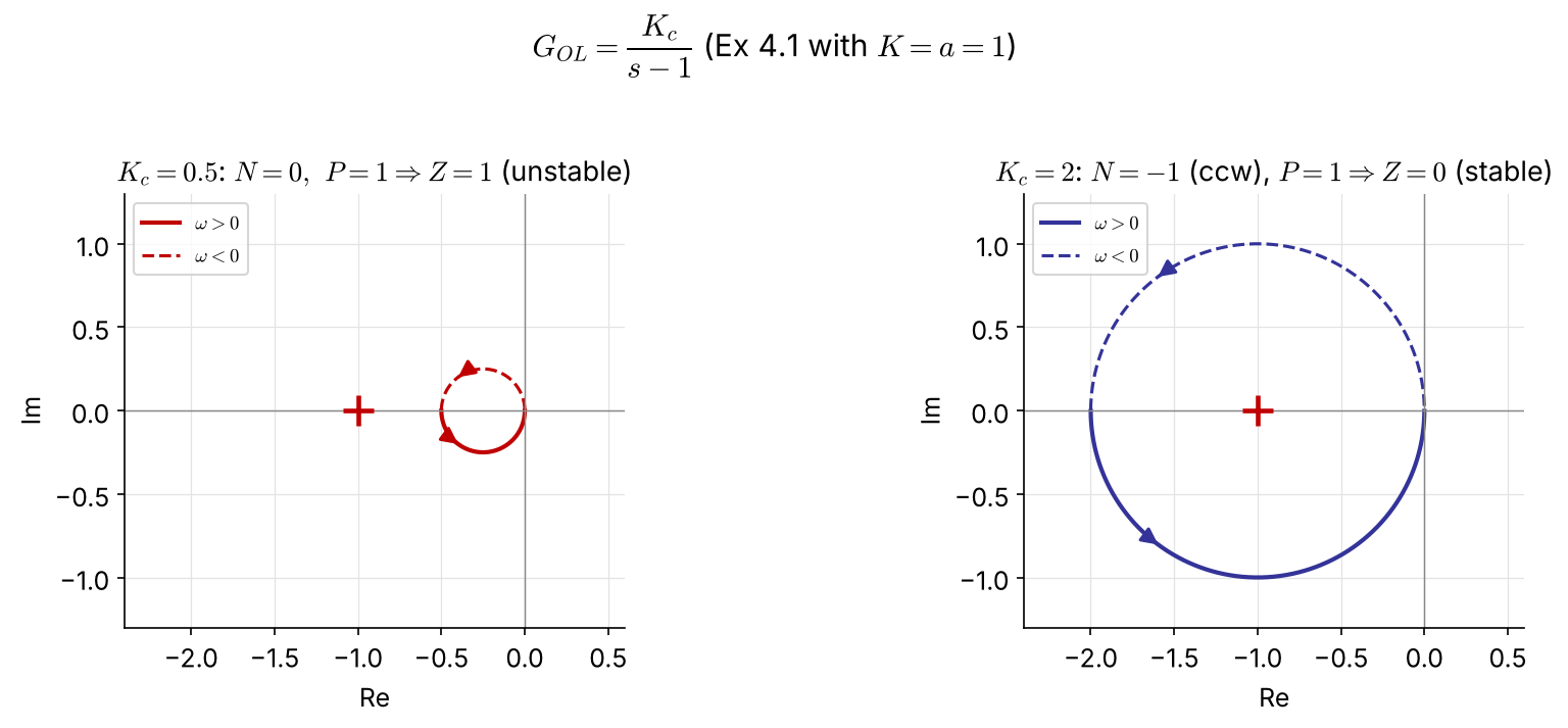
\(K_c/(s-1)\) is a circle of diameter \(K_c\) through \(0\) and \(-K_c\), traversed counterclockwise. \(P=1\), so stability needs \(N=-1\): the circle must enclose \(-1\) ⇒ \(K_c>1\) — exactly Ex 4.1 (\(K_cK>a\)). The Bode criterion cannot be used here (\(P\neq0\)).

Gain and phase margins
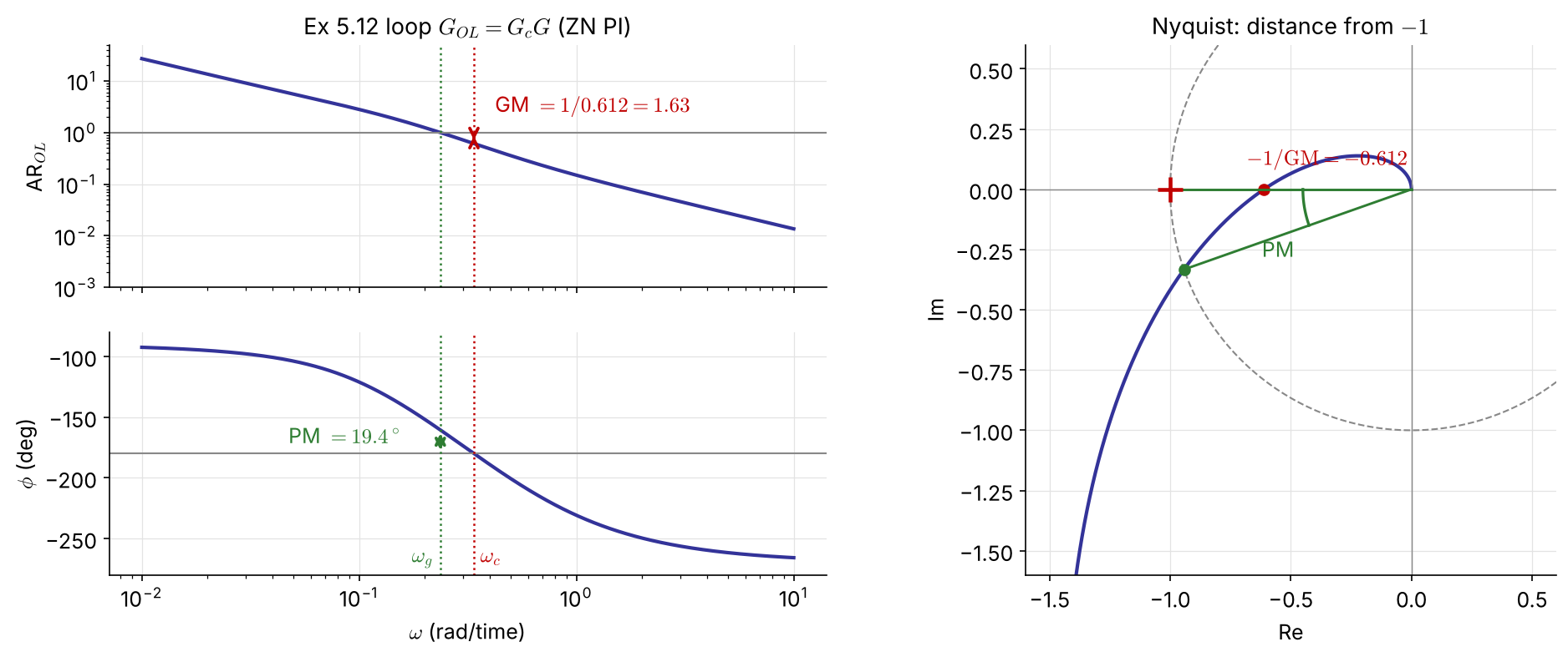
Gain margin (at \(\omega_c\), where \(\angle G_{OL}=-180^\circ\)) \[ \mathrm{GM}=\frac{1}{|G_{OL}(j\omega_c)|} \]

Phase margin (at \(\omega_g\), where \(|G_{OL}|=1\)) \[ \mathrm{PM}=180^\circ+\angle G_{OL}(j\omega_g) \]

What the margins protect against

GM — factor by which the loop gain can grow before instability → safeguard against gain (model) error

Typical spec: GM > 2 (6 dB)

GM \(=1/|G_{OL}(j\omega_c)|\) is the distance from \(-1\) along the real axis

PM — extra phase lag tolerated at \(\omega_g\) → safeguard against dead-time error

Typical spec: PM > 30° (often 45°)

Extra delay that destabilizes: FIX \[ \theta_{\max}=\frac{\mathrm{PM}\ (\text{rad})}{\omega_g} \]

  • If several crossings: take the one closest to \(-1\) (largest \(|G_{OL}|\)) for GM, the smallest PM. Low-order minimum-phase plants may have GM \(=\infty\).
  • Lowering \(\omega_g\) (smaller bandwidth, slower loop) tolerates larger delay errors. Ex 5.12: \(\theta_{\max}=0.339/0.236=1.4\) s.

Phase margin and damping NEW

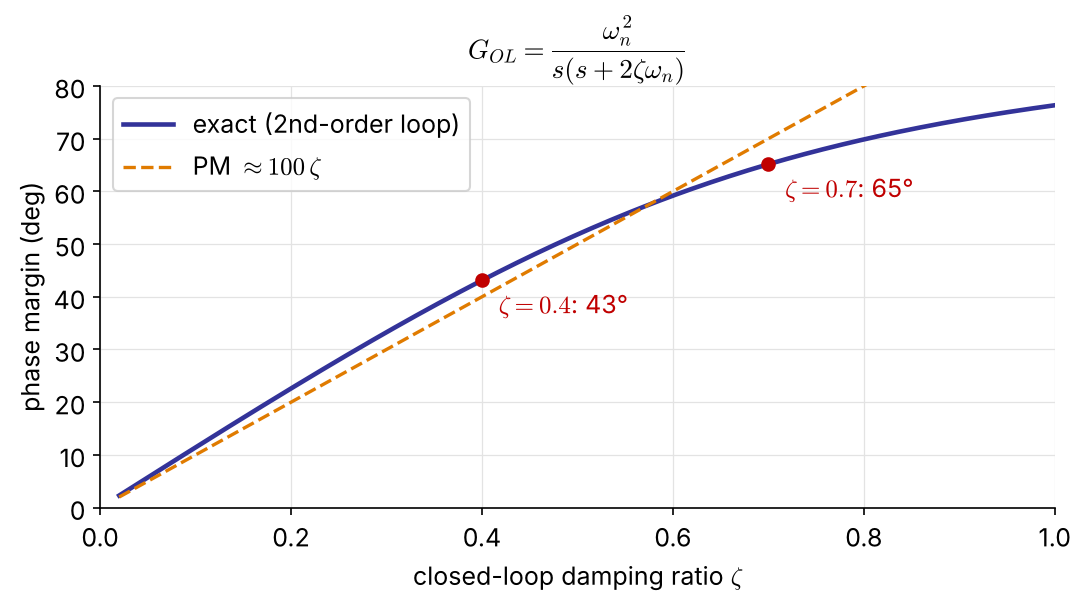
For a loop that behaves like \(\dfrac{\omega_n^2}{s(s+2\zeta\omega_n)}\):

\[ \mathrm{PM}=\tan^{-1}\!\frac{2\zeta}{\sqrt{\sqrt{1+4\zeta^4}-2\zeta^2}} \;\approx\;100\,\zeta\ (\text{deg}) \]

PM 45° ↔︎ \(\zeta\approx0.4\) (overshoot ≈ 25 %)

PM 65° ↔︎ \(\zeta\approx0.7\) (overshoot ≈ 5 %)

A small PM means an oscillatory closed loop — the bridge to the \(\zeta\)-based root-locus design of Ch 4.

Example 5.12   Ziegler–Nichols PI for the inverse-response process
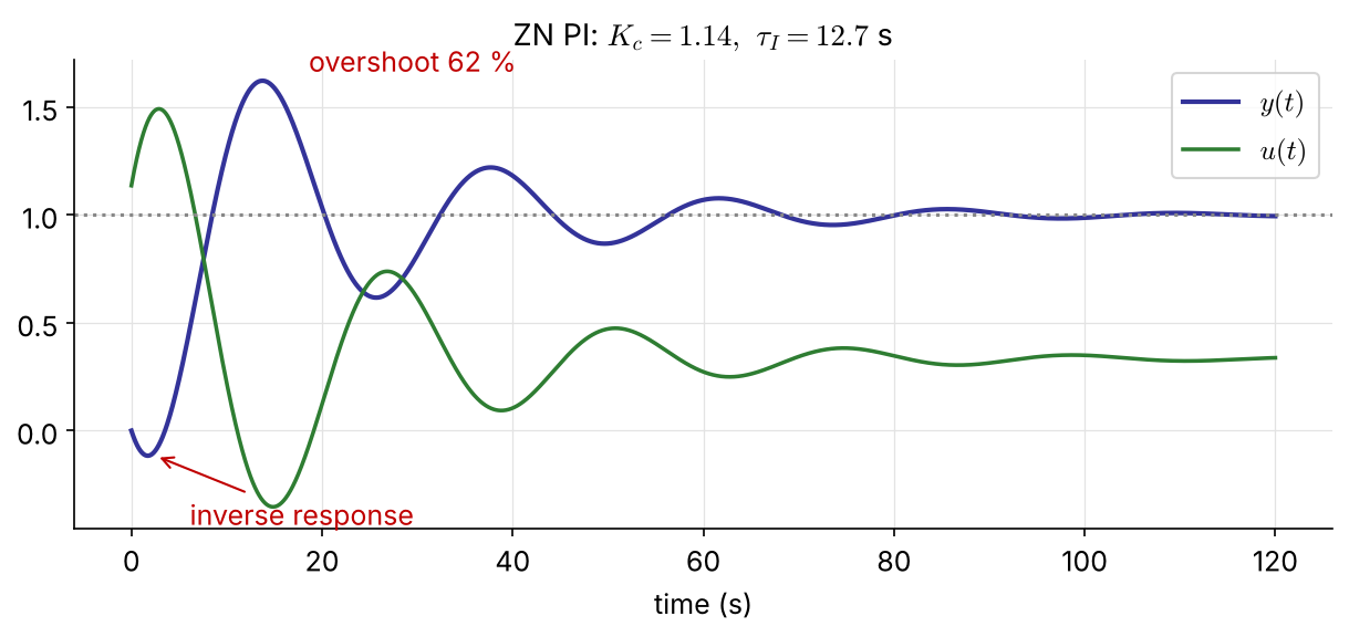
\(G_c=K_c\left(1+\dfrac{1}{\tau_Is}\right)\) removes the P-control offset.

ZN settings from Ex 5.11 (\(K_u=2.5,\ P_u=15.2\) s):

\[ K_c=\frac{K_u}{2.2}=1.14,\qquad \tau_I=\frac{P_u}{1.2}=12.7\ \text{s} \]

GM \(=1.63\), PM \(=19.4^\circ\)
— too small (GM > 2, PM > 30°)

→ 62 % overshoot, slow-decaying oscillation

ZN tunings are deliberately “aggressive” (quarter-decay); use them only as a starting point.

Margins in code

import numpy as np, control as ct

G = ct.tf([-6, 3], np.polymul([10, 1], [5, 1]))
gm, pm, wc, wg = ct.margin(G)          # P control with Kc = 1
Ku, Pu = gm, 2*np.pi/wc                # 2.5, 15.2 s

Kc, tI = Ku/2.2, Pu/1.2                # Ziegler-Nichols PI
L = Kc*ct.tf([tI, 1], [tI, 0])*G
gm, pm, wc, wg = ct.margin(L)          # GM 1.63, PM 19.4 deg
theta_max = np.radians(pm)/wg          # 1.43 s of extra dead time
ct.bode_plot(L, display_margins=True)
G = tf([-6 3], conv([10 1],[5 1]));
[Ku,~,wc] = margin(G);   Pu = 2*pi/wc;      % 2.5, 15.2 s

Kc = Ku/2.2;   tI = Pu/1.2;                 % Ziegler-Nichols PI
L = Kc*tf([tI 1],[tI 0])*G;
[GM,PM,wc,wg] = margin(L)                   % 1.63, 19.4 deg
theta_max = PM*pi/180/wg                    % 1.43 s
margin(L)                                   % Bode plot with margins marked

5.4 Controller Design

Choosing \(K_c\) without trial and error

Write the loop as \(\;1+G_{OL}=1+K_cG^*=0\), where \(G^*\) contains everything except \(K_c\) (process, valve, sensor, and the \(\tau_I,\tau_D\) terms of the controller).

From a GM spec

\(\angle K_c=0\), so \(G^*\) and \(G_{OL}\) share \(\omega_c\):

\[ K_{cu}=\frac{1}{|G^*(j\omega_c)|},\qquad K_c=\frac{K_{cu}}{\mathrm{GM}} \]

From a PM spec

Find \(\omega_g\) where \(\angle G^*=-180^\circ+\mathrm{PM}\)
(e.g. \(-135^\circ\) for 45°):

\[ K_c=\frac{1}{|G^*(j\omega_g)|} \]

Compute both and take the smaller \(K_c\), which satisfies both specs. One Bode plot of \(G^*\) does it all.

Example 5.13   Retuning Ex 5.12 for GM ≥ 2 and PM ≥ 45° NEW
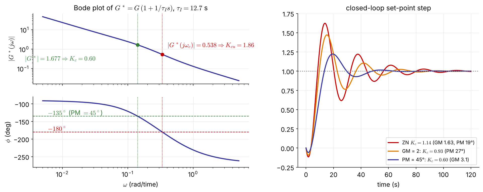
Keep \(\tau_I=12.7\) s: \(\;G^*=G\,(1+1/\tau_Is)\), \(\ \omega_c=0.338\), \(\ K_{cu}=1.86\)

  • GM \(=2\) → \(K_c=0.93\) (but PM only 27°)
  • PM \(=45^\circ\) → \(\omega_g=0.142\), \(\ K_c=0.60\) (GM 3.1)

\(K_c=0.60\) meets both specs: overshoot 62 % → 22 %, settles in 45 s instead of 89 s

Example 5.13 in code

tI = Pu/1.2
Gs = ct.tf([tI, 1], [tI, 0])*G                  # G* = everything except Kc

Kcu = ct.margin(Gs)[0]                          # 1.86
Kc_GM = Kcu/2                                   # GM = 2   -> 0.93

w = np.logspace(-3, 1, 100000)
g = Gs(1j*w)
phase = np.degrees(np.unwrap(np.angle(g)))
i = np.argmin(abs(phase - (-180 + 45)))         # phase = -135 deg
Kc_PM = 1/abs(g[i])                             # PM = 45 deg -> 0.60

Kc = min(Kc_GM, Kc_PM)
print(ct.margin(Kc*Gs), ct.step_info(ct.feedback(Kc*Gs, 1)))
tI = Pu/1.2;
Gs = tf([tI 1],[tI 0])*G;                       % G* = everything except Kc

Kcu = margin(Gs);   Kc_GM = Kcu/2;              % 1.86 -> 0.93

w = logspace(-3, 1, 1e5);
[m, p] = bode(Gs, w);   m = squeeze(m);   p = squeeze(p);
[~, i] = min(abs(p + 135));                     % phase = -135 deg
Kc_PM = 1/m(i)                                  % 0.60

Kc = min(Kc_GM, Kc_PM);
margin(Kc*Gs), stepinfo(feedback(Kc*Gs, 1))

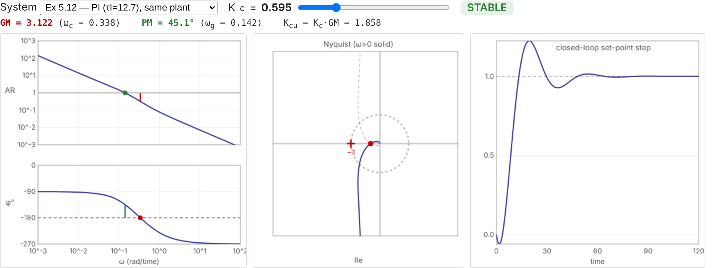
Interactive: move \(K_c\), watch the margins NEW
A final word: frequency response or root locus?

They complement each other; a design decision is often made only after both.

Root locus (Ch 4)

  • shows the transient response and how it moves with \(K_c\)
  • needs a fairly accurate model
  • does not handle dead time well

Frequency response (Ch 5)

  • relative stability: GM, PM; dead time exactly
  • Bode plot can come from experiments (sine or pulse tests) — no model needed, or a check of one
  • several crossovers: use Nyquist, not Bode alone
Task MATLAB Python (control)
Bode / Nyquist bode(G), nyquist(G) ct.bode_plot(G), ct.nyquist_plot(G)
dead time tf(..., 'InputDelay', θ) G(1j*w)*np.exp(-1j*w*θ)
margins [GM,PM,wc,wg] = margin(L) gm, pm, wc, wg = ct.margin(L)

Problem #1   (homework) NEW

\[ G_p=\frac{2e^{-s}}{10s+1},\qquad G_c=K_c\left(1+\frac{1}{\tau_Is}\right),\quad \tau_I=10 \]

  1. Show that \(\tau_I=10\) makes \(G_{OL}\) a pure integrator with dead time. Sketch its Bode plot by hand.

  2. Find the phase crossover \(\omega_c\) and the ultimate gain \(K_{cu}\) analytically.

  3. Find \(K_c\) for PM \(=45^\circ\). What is the resulting GM? Comment on the result.

  4. Check (b)–(c) with ct.margin and simulate the set-point response.

Resources

Appendix

General frequency response: derivation

Stable \(G=Q/P\), input \(A\sin\omega t\): \(\;Y(s)=\dfrac{Q(s)}{P(s)}\dfrac{A\omega}{(s+j\omega)(s-j\omega)}\)

All roots of \(P\) have negative real parts, so their terms decay. At large times only the input poles remain:

\[ Y_\infty(s)=\frac{a}{s+j\omega}+\frac{a^*}{s-j\omega},\qquad a=(s+j\omega)Y(s)\big|_{s=-j\omega}=\frac{AG(-j\omega)}{-2j} \]

With \(G(\pm j\omega)=|G(j\omega)|e^{\pm j\phi}\):

\[ \frac{y_\infty(t)}{A}=|G(j\omega)|\left(\frac{e^{-j(\omega t+\phi)}}{-2j}+\frac{e^{j(\omega t+\phi)}}{2j}\right)=|G(j\omega)|\sin(\omega t+\phi),\qquad \phi=\angle G(j\omega) \]

Resonance of the second-order system

\[ \frac{d}{d\omega}\Big[(1-\tau^2\omega^2)^2+(2\zeta\tau\omega)^2\Big]=0 \;\Rightarrow\;\tau^2\omega_r^2=1-2\zeta^2 \]

\[ M_{p\omega}=|G(j\omega_r)|=\frac{K}{\sqrt{(2\zeta^2)^2+4\zeta^2(1-2\zeta^2)}}=\frac{K}{2\zeta\sqrt{1-\zeta^2}} \]

A real \(\omega_r\) requires \(1-2\zeta^2>0\), i.e. \(\zeta<1/\sqrt2\).

\(\zeta\) 0.2 0.4 0.6
\(\tau\omega_r\) 0.96 0.82 0.53
\(M_{p\omega}/K\) 2.55 (8.1 dB) 1.36 (2.7 dB) 1.04 (0.4 dB)