1. Mathematical Preliminaries and Dynamic Response
Before we design controllers we need a language for how processes respond in time: models in deviation variables, the Laplace transform, and transfer functions whose poles tell us the shape of the response without solving for it.
| Section | Topic | Key result |
|---|---|---|
| 1.1 | process models, deviation variables, linearization | linear ODEs with zero initial conditions |
| 1.2 | Laplace transform | table look-up, initial- and final-value theorems |
| 1.3 | partial-fraction expansion | each pole gives one term of \(f(t)\) |
| 1.4 | transfer functions, poles and zeros | poles fix the time dependence, zeros the coefficients |
| 1.5–1.6 | first- and second-order systems | \(\tau\), \(K\), \(\zeta\); overshoot, decay ratio, settling time |
| 1.7–1.9 | dead time, higher order, zeros | Padé, FOPDT approximation, inverse response |
Any linear model breaks into first-order terms by partial fractions, and complex-conjugate pairs combine into second-order terms, so first- and second-order systems are all we need to study in detail.
Mass balance of a well-mixed tank: \[ \tau\frac{dc}{dt}=c_{in}-c,\qquad c(0)=c_0,\qquad \tau=\frac{V}{q} \]
Define deviation variables from the initial steady state: \(\bar c=c-c_0\), \(\bar c_{in}=c_{in}-c_0\).
\[ \tau\frac{d\bar c}{dt}+\bar c=\bar c_{in},\qquad \bar c(0)=0 \]
Why deviation variables? The initial condition becomes zero, so the Laplace transform of the model contains no initial-condition terms and gives a clean input–output ratio. For reference, the solution is the convolution \(\bar c(t)=\dfrac1\tau\displaystyle\int_0^t\bar c_{in}(\alpha)e^{-(t-\alpha)/\tau}d\alpha\).

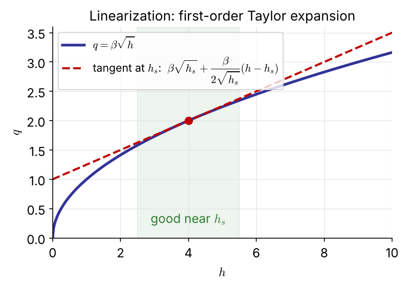
\[ A\frac{dh}{dt}=q_i-\beta\sqrt h,\qquad h(0)=h_s \]
Steady state: \(0=q_{i,s}-\beta\sqrt{h_s}\). Taylor-expand \(\sqrt h\) about \(h_s\): \[ A\frac{dh}{dt}\simeq q_i-\beta\left[\sqrt{h_s}+\frac{1}{2\sqrt{h_s}}(h-h_s)\right] \]
Subtract the steady state and use \(\bar q_i=q_i-q_{i,s}\), \(\bar h=h-h_s\) FIX: \[ A\frac{d\bar h}{dt}+\frac{\beta}{2\sqrt{h_s}}\bar h=\bar q_i,\qquad \bar h(0)=0 \]
General case (one state \(y\), inputs \(\mathbf u\)): with \(y'=y-y_s\), \(\mathbf u'=\mathbf u-\mathbf u_s\), \[ \frac{dy'}{dt}=\left.\frac{\partial f}{\partial y}\right|_s y'+\nabla_{\mathbf u}^Tf\big|_s\,\mathbf u' \] The model is accurate only near the operating point.
\[ V\frac{dc}{dt}=q\,c_i-q\,c \qquad (q \text{ and } c_i \text{ both vary with time}) \]
The product terms are nonlinear. Expand about \((q_s,c_{i,s},c_s)\): \[ qc_i\simeq q_sc_{i,s}+c_{i,s}\,q'+q_s\,c_i' \] \[ qc\simeq q_sc_s+c_s\,q'+q_s\,c' \] Subtract the steady state \(0=q_s(c_{i,s}-c_s)\): \[ V\frac{dc'}{dt}=q_s(c_i'-c')+(c_{i,s}-c_s)\,q' \]
At steady state \(c_s=c_{i,s}\), so the flow term vanishes: \[ \frac{V}{q_s}\frac{dc'}{dt}+c'=c_i' \] To first order, a flow change does not move the concentration; only \(c_i\) does. NEW
\[ \rho C_pV\frac{dT}{dt}=\rho C_pq(T_i-T)+UA(T_H-T) \] With \(\tau=V/q\) and \(\kappa=UA/(\rho C_pq)\), in deviation variables: \[ \tau\frac{d\bar T}{dt}+(1+\kappa)\bar T=\bar T_i+\kappa\bar T_H \]
Pole-zero form \[ T(s)=\frac{K_i}{s+a}T_i(s)+\frac{K_H}{s+a}T_H(s) \] \(a=\dfrac{1+\kappa}{\tau},\ K_i=\dfrac1\tau,\ K_H=\dfrac\kappa\tau\)
Time-constant form (used in control) \[ T(s)=\frac{K_d}{\tau_ps+1}T_i(s)+\frac{K_p}{\tau_ps+1}T_H(s) \] \(\tau_p=\dfrac{\tau}{1+\kappa},\ K_d=\dfrac1{1+\kappa},\ K_p=\dfrac{\kappa}{1+\kappa}\)
One output, two inputs: the heater temperature \(T_H\) will be our manipulated variable, the inlet temperature \(T_i\) a disturbance. Both see the same pole \(-1/\tau_p\).
\[ V\frac{dc_A}{dt}=q(c_{Ai}-c_A)-Vk(T)\,c_A \] \[ \rho VC_p\frac{dT}{dt}=\rho qC_p(T_i-T)+(-\Delta H_R)Vk(T)c_A+UA(T_c-T) \] \(k(T)c_A\) is nonlinear in both states. With \(q\), \(c_{Ai}\), \(T_i\) constant, linearize (\(k_s'=k_sE/RT_s^2\)): \[ \frac{d}{dt}\begin{bmatrix}c_A'\\T'\end{bmatrix}=\begin{bmatrix}a_{11}&a_{12}\\a_{21}&a_{22}\end{bmatrix}\begin{bmatrix}c_A'\\T'\end{bmatrix}+\begin{bmatrix}0\\b_2\end{bmatrix}T_c' \]
\(a_{11}=-\dfrac qV-k_s,\quad a_{12}=-k_s'c_{As},\quad a_{21}=\dfrac{(-\Delta H_R)k_s}{\rho C_p}\) \(a_{22}=-\dfrac qV-\dfrac{UA}{\rho VC_p}+\dfrac{(-\Delta H_R)k_s'c_{As}}{\rho C_p},\quad b_2=\dfrac{UA}{\rho VC_p}\)
\[ \frac{C_A'(s)}{T_c'(s)}=\frac{a_{12}b_2}{(s-a_{11})(s-a_{22})-a_{12}a_{21}} \] NEW second order: the two balances are coupled.
For the CSTR of Example 1.3, find all the approximate transfer functions relating the outputs \(c_A\) and \(T\) to the inputs \(c_{A,i}\), \(T_i\) and \(T_c\).
Show that all six transfer functions share one denominator, and explain why.
Hint: write the Laplace-transformed linear model as \((s\mathbf I-\mathbf A)\mathbf x=\mathbf B\mathbf u\) and solve with Cramer’s rule; the denominator is \(\det(s\mathbf I-\mathbf A)\).
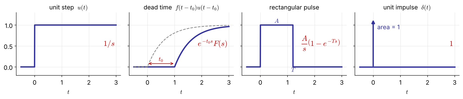
\[ \mathcal L[f(t)]=\int_0^\infty f(t)e^{-st}dt=F(s),\qquad f(t)=\mathcal L^{-1}[F(s)]=\frac{1}{2\pi j}\int_{\gamma-j\infty}^{\gamma+j\infty}F(s)e^{st}ds \]
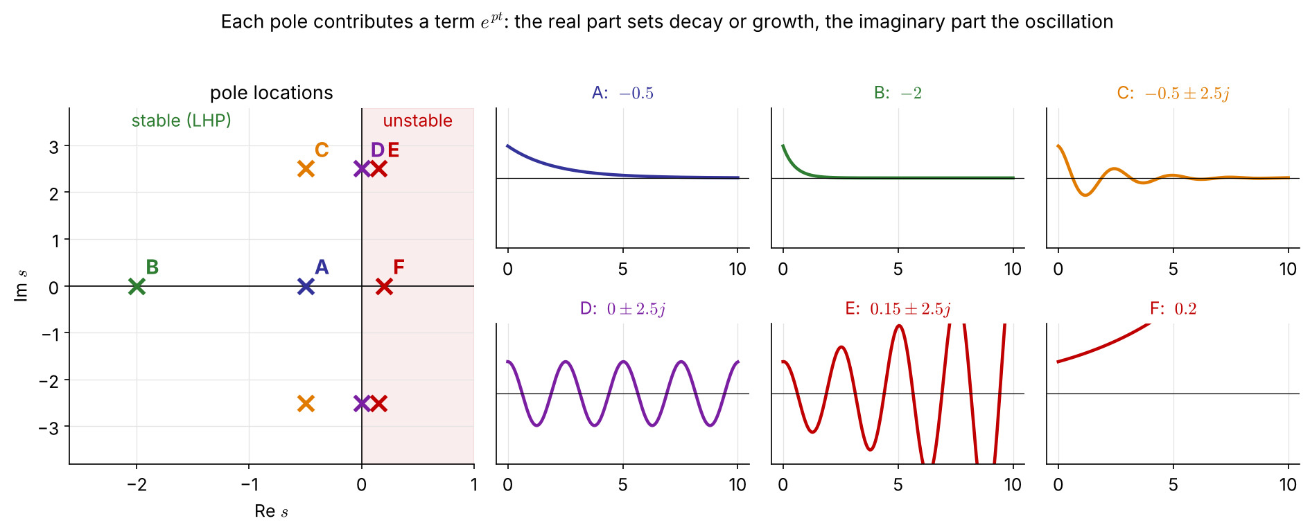
The real goal: predict the time response without the inverse transform. The answer lies in the roots of the characteristic equation (§1.4).
| \(f(t)\) | \(F(s)\) |
|---|---|
| \(\delta(t)\) (unit impulse) | \(1\) |
| \(u(t)\) (unit step) | \(\dfrac1s\) |
| \(t\) (ramp) | \(\dfrac1{s^2}\) |
| \(t^{n-1}/(n-1)!\) | \(\dfrac1{s^n}\) |
| \(e^{-at}\) | \(\dfrac1{s+a}\) |
| \(t^{n-1}e^{-at}/(n-1)!\) | \(\dfrac1{(s+a)^n}\) |
| \(\sin\omega t\), \(\cos\omega t\) | \(\dfrac{\omega}{s^2+\omega^2}\), \(\dfrac{s}{s^2+\omega^2}\) |
| \(e^{-at}\sin\omega t\), \(e^{-at}\cos\omega t\) | \(\dfrac{\omega}{(s+a)^2+\omega^2}\), \(\dfrac{s+a}{(s+a)^2+\omega^2}\) |
| Operation | Transform |
|---|---|
| \(\dfrac{df}{dt}\) | \(sF(s)-f(0)\) |
| \(\dfrac{d^2f}{dt^2}\) | \(s^2F(s)-sf(0)-f'(0)\) |
| \(\displaystyle\int_0^tf\,dt\) | \(\dfrac{F(s)}s\) |
| \(f(t-t_0)u(t-t_0)\) | \(e^{-st_0}F(s)\) |
| \(e^{-at}f(t)\) | \(F(s+a)\) |
Derivation by integration by parts, e.g. \(\mathcal L[df/dt]=fe^{-st}\big|_0^\infty+s\int_0^\infty fe^{-st}dt=sF(s)-f(0)\). With deviation variables all \(f^{(k)}(0)=0\), so \(d/dt\to s\) and \(\int dt\to1/s\).
Try: derive \(\mathcal L[\cos\omega t]\) from \(\cos\omega t=(e^{j\omega t}+e^{-j\omega t})/2\).
Values of \(f(t)\) at the two extremes without the inverse transform:
\[ \lim_{t\to0^+}f(t)=\lim_{s\to\infty}sF(s),\qquad\qquad \lim_{t\to\infty}f(t)=\lim_{s\to0}sF(s) \]
Proof of the final value: \(\displaystyle\lim_{s\to0}\int_0^\infty\frac{df}{dt}e^{-st}dt=\int_0^\infty df=f(\infty)-f(0)\), and the left side is \(\lim_{s\to0}[sF(s)-f(0)]\).
The final-value theorem holds only if \(f(\infty)\) exists: all poles of \(sF(s)\) must lie in the left half-plane. FIX
Example 1.4 What is \(f(\infty)\)?
\(F=\dfrac{6(s-2)(s+2)}{s(s+1)(s+3)(s+4)}\): \(\ sF(0)=\dfrac{6(-2)(2)}{(3)(4)}=\) \(-2\)
\(F=\dfrac1{s-2}\), i.e. \(f=e^{2t}\): \(\ sF(0)=0\), but \(f\to\infty\): theorem not applicable (pole at \(+2\)).
\(F=\dfrac{6(s+3)}{s^3+s^2-4s-4}=\dfrac{6(s+3)}{(s+1)(s+2)(s-2)}\): again a pole at \(+2\); \(f(\infty)\) does not exist.
\[ F(s)=\frac{q(s)}{p(s)}=\frac{\alpha_1}{s+a_1}+\frac{\alpha_2}{s+a_2}+\cdots+\frac{\alpha_n}{s+a_n} \quad\Rightarrow\quad f(t)=\sum_i\alpha_ie^{-a_it} \]
\(-a_i\) are the roots of \(p(s)=0\) (order \(n\) > order of \(q\)). Heaviside’s cover-up rule:
\[ \alpha_i=(s+a_i)\left.\frac{q(s)}{p(s)}\right|_{s=-a_i} \]
\(s^3+s^2-4s-4=(s+1)(s+2)(s-2)\). Two numerators, same denominator:
| \(\dfrac{6s^2-12}{(s+1)(s+2)(s-2)}\) | \(\dfrac{6s}{(s+1)(s+2)(s-2)}\) | |
|---|---|---|
| \(\alpha_1=\left.\dfrac{q}{(s+2)(s-2)}\right\vert_{-1}\) | \(\dfrac{-6}{-3}=2\) | \(\dfrac{-6}{-3}=2\) |
| \(\alpha_2=\left.\dfrac{q}{(s+1)(s-2)}\right\vert_{-2}\) | \(\dfrac{12}{4}=3\) | \(\dfrac{-12}{4}=-3\) |
| \(\alpha_3=\left.\dfrac{q}{(s+1)(s+2)}\right\vert_{2}\) | \(\dfrac{12}{12}=1\) | \(\dfrac{12}{12}=1\) |
| \(f(t)\) | \(2e^{-t}+3e^{-2t}+e^{2t}\) | \(2e^{-t}-3e^{-2t}+e^{2t}\) |
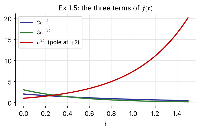
Same three exponentials, different coefficients: the numerator changes only the weights.

The same procedure gives \(\dfrac{6}{(s+1)(s+2)(s+3)}=\dfrac3{s+1}-\dfrac6{s+2}+\dfrac3{s+3}\).
\[ F(s)=\frac{s+5}{s^2+4s+13},\qquad s^2+4s+13=0\ \Rightarrow\ s=-2\pm3j \]
Method 1: cover-up with complex numbers \[ \alpha=\left.\frac{s+5}{s-(-2-3j)}\right|_{s=-2+3j}=\frac{3+3j}{6j}=\frac{1-j}{2},\quad \alpha^*=\frac{1+j}{2} \] \[ f(t)=\tfrac{1-j}{2}e^{(-2+3j)t}+\tfrac{1+j}{2}e^{(-2-3j)t} \] Euler’s formula collects the terms into real functions.
Method 2: complete the square (faster) \[ \frac{s+5}{(s+2)^2+3^2}=\frac{s+2}{(s+2)^2+3^2}+\frac{3}{(s+2)^2+3^2} \] \[ f(t)=e^{-2t}(\cos3t+\sin3t) \]
Phase-lag form (the one we use): \(\ \cos3t+\sin3t=\sqrt2\sin(3t+\phi),\ \phi=\tan^{-1}1=\pi/4\), so \(f(t)=\sqrt2\,e^{-2t}\sin(3t+\pi/4)\). Roots \(-a\pm bj\) always give \(e^{-at}\) times an oscillation of frequency \(b\)
\[ \frac{2}{(s+1)^3(s+2)}=\frac{\alpha_1}{s+1}+\frac{\alpha_2}{(s+1)^2}+\frac{\alpha_3}{(s+1)^3}+\frac{\alpha_4}{s+2} \]
\(\alpha_4=\left.\dfrac2{(s+1)^3}\right|_{-2}=-2\). Multiply by \((s+1)^3\): \[ \frac2{s+2}=\alpha_1(s+1)^2+\alpha_2(s+1)+\alpha_3+\alpha_4\frac{(s+1)^3}{s+2} \] Set \(s=-1\), then differentiate and set \(s=-1\) again:
\(\alpha_3=2,\quad \alpha_2=\left.-\dfrac2{(s+2)^2}\right|_{-1}=-2,\quad \alpha_1=\dfrac12\left.\dfrac4{(s+2)^3}\right|_{-1}=2\)
\[ f(t)=2\left[\left(1-t+\tfrac{t^2}2\right)e^{-t}-e^{-2t}\right] \]
In general \[ \mathcal L^{-1}\left[\sum_{k=1}^n\frac{\alpha_k}{(s+a)^k}\right]=\left[\alpha_1+\alpha_2t+\cdots+\frac{\alpha_nt^{n-1}}{(n-1)!}\right]e^{-at} \] Still based on the root \(-a\), but the polynomial in \(t\) makes it decay more slowly.
import sympy as sp
s, t = sp.symbols('s t'); tp = sp.Symbol('t', positive=True)
for F in [(6*s**2 - 12)/(s**3 + s**2 - 4*s - 4), # Ex 1.5
(s + 5)/(s**2 + 4*s + 13), # Ex 1.6
2/((s + 1)**3*(s + 2))]: # Ex 1.7
print(sp.apart(F, s), ' -> ', sp.inverse_laplace_transform(F, s, tp))
import numpy as np, scipy.signal as sig
r, p, k = sig.residue([6, 0, -12], [1, 1, -4, -4]) # residues, poles, direct term
print(np.round(r, 4), np.round(p, 4)) # [3, 2, 1] at [-2, -1, 2]Check your answers with sympy.inverse_laplace_transform or MATLAB ilaplace.
For a linear ODE with zero initial conditions (\(n\ge m\)) \[ a_ny^{(n)}+\cdots+a_1y'+a_0y=b_mx^{(m)}+\cdots+b_1x'+b_0x \] the Laplace transform gives the transfer function, the ratio of output to input: \[ G(s)=\frac{Y(s)}{X(s)}=\frac{b_ms^m+\cdots+b_1s+b_0}{a_ns^n+\cdots+a_1s+a_0}=\frac{Q(s)}{P(s)} \]
Pole-zero form \[ G(s)=\frac{b_m}{a_n}\frac{(s-z_1)\cdots(s-z_m)}{(s-p_1)\cdots(s-p_n)} \] \(P(s)\) is the characteristic polynomial; its roots are the poles, the roots of \(Q(s)\) the zeros.
Time-constant form (real roots) \[ G(s)=K\frac{(\tau_as+1)\cdots(\tau_ms+1)}{(\tau_1s+1)\cdots(\tau_ns+1)} \] Steady-state gain: final change of \(y\) per unit step in \(x\), \(K=\lim_{s\to0}sG(s)\dfrac1s=G(0)=\dfrac{b_0}{a_0}\)
From §1.1, \(\ \tau\dfrac{d\bar c}{dt}+\bar c=\bar c_{in}\ \Rightarrow\ (\tau s+1)C(s)=C_{in}(s)\ \Rightarrow\ G(s)=\dfrac{C(s)}{C_{in}(s)}=\dfrac{1}{\tau s+1}\), one pole at \(-1/\tau\).
Unit step \(C_{in}=1/s\) \[ C=\frac1{(\tau s+1)s}=\frac1s-\frac1{s+1/\tau} \] \[ \bar c(t)=1-e^{-t/\tau} \]
Unit impulse \(C_{in}=1\) \[ C=\frac{1}{\tau s+1}=\frac1\tau\frac1{s+1/\tau} \] \[ \bar c(t)=\frac1\tau e^{-t/\tau} \]
Without specifying the input we already know \(\bar c(t)\) must contain \(e^{-t/\tau}\): that is what the pole tells us.
\[ a_1\frac{dy}{dt}+a_0y=bx(t)\quad\Rightarrow\quad \tau\frac{dy}{dt}+y=Kx(t),\qquad G(s)=\frac{Y(s)}{X(s)}=\frac{K}{\tau s+1} \]
\(\tau=a_1/a_0\): time constant (시간상수), \(K=b/a_0\): steady-state gain (정상상태 이득), one real pole at \(-1/\tau\).
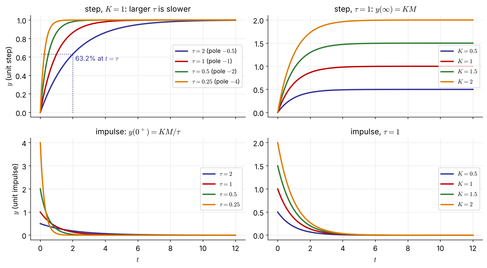
Step \(x=Mu(t)\): \[ Y=\frac{KM}{s(\tau s+1)}\ \Rightarrow\ y(t)=KM\left(1-e^{-t/\tau}\right) \] Impulse \(x=M\delta(t)\): \[ y(t)=\frac{KM}{\tau}e^{-t/\tau} \] Final value check: \(\lim_{s\to0}s\dfrac{KM}{s(\tau s+1)}=KM\).
| \(t\) | \(y/KM=1-e^{-t/\tau}\) |
|---|---|
| \(\tau\) | 0.632 |
| \(2\tau\) | 0.865 |
| \(3\tau\) | 0.950 |
| \(4\tau\) | 0.982 |
| \(5\tau\) | 0.993 |
After \(3\tau\) within 5%, after \(5\tau\) within 1%: “settled”.
The larger the time constant, the slower the response. The larger the gain, the more sensitive the output to the input.
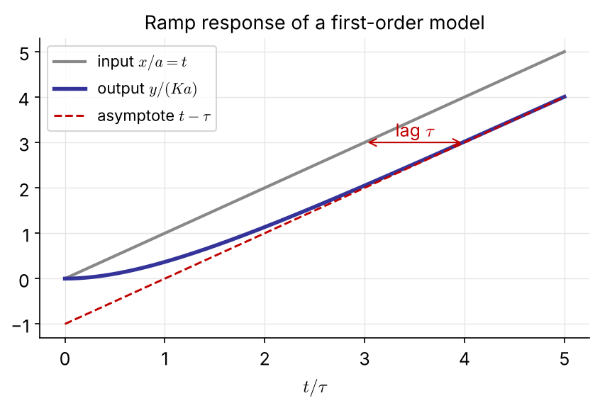
Ramp \(x=at\), \(X=a/s^2\): \[ Y=\frac{Ka}{s^2(\tau s+1)}=\frac{Ka\tau^2}{\tau s+1}-\frac{Ka\tau}{s}+\frac{Ka}{s^2} \] \[ y(t)=Ka\tau\left(e^{-t/\tau}-1\right)+Kat \]
\(\to Ka(t-\tau)\) for \(t\gg\tau\): the output lags the input by \(\tau\).
Integrating process (\(a_0=0\)): \[ \frac{dy}{dt}=K_Ix(t)\ \Rightarrow\ G(s)=\frac{K_I}{s} \] a pole at the origin.
\(A\dfrac{d\bar h}{dt}=\bar q_{in}-\bar q\ \Rightarrow\ H(s)=\dfrac1A\dfrac{Q_{in}(s)-Q(s)}{s}\)
A step input gives a ramp; an impulse is not forgotten, the level keeps whatever was added. Not self-regulating: levels need control.
\(\tau_1\dfrac{d\bar c_1}{dt}+\bar c_1=\bar c_i,\quad \tau_2\dfrac{d\bar c_2}{dt}+\bar c_2=\bar c_1\) \[ \frac{C_2(s)}{C_i(s)}=\frac{1}{(\tau_1s+1)(\tau_2s+1)} \]
\(\tau_1=V_1/q=2\) min, \(\ \tau_2=V_2/q=1.5\) min
Feed: \(c_i=6\) for \(0<t<0.25\) min, otherwise 1, so \(\bar c_i\) is a pulse of height 5: \[ C_i(s)=\frac5s\left(1-e^{-s/4}\right)\quad\text{or, as an impulse,}\quad C_i(s)=\frac54 \] \[ C_2(s)=\frac{5(1-e^{-s/4})}{s(2s+1)(1.5s+1)}\quad\text{or}\quad\frac{5/4}{(2s+1)(1.5s+1)} \]
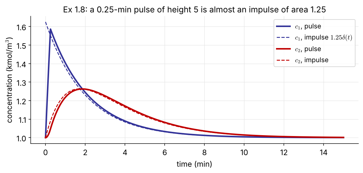
The original MATLAB script used pulselength = 1.25, a pulse 5× too long. FIX
For Example 1.8, carry out the inverse transforms:
the impulse response \(\bar c_2(t)\) for \(C_i=5/4\);
the pulse response \(\bar c_2(t)\), using the dead-time property for the factor \(e^{-s/4}\).
Plot both together with \(\bar c_1(t)\) and compare with the figure on the previous slide.
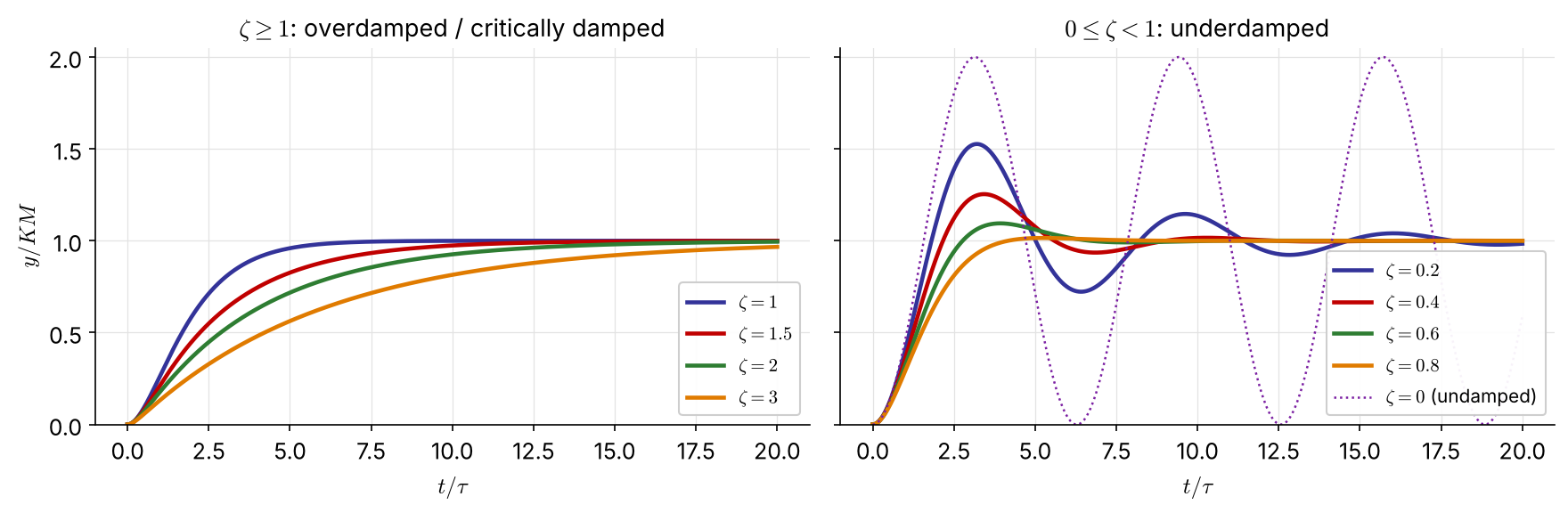
\[ \tau^2\frac{d^2y}{dt^2}+2\zeta\tau\frac{dy}{dt}+y=Kx(t)\quad\Rightarrow\quad G(s)=\frac{K}{\tau^2s^2+2\zeta\tau s+1}=\frac{K\omega_n^2}{s^2+2\zeta\omega_ns+\omega_n^2} \]
\(\tau\): natural period, \(\omega_n=1/\tau\): natural frequency, \(\zeta\): damping ratio (감쇠계수), \(K\): steady-state gain. Poles: \[ p_{1,2}=-\frac{\zeta}{\tau}\pm\frac{\sqrt{\zeta^2-1}}{\tau}\qquad(\text{stable only if }\zeta>0,\ \text{since }\tau>0) \]
| \(\zeta\) | poles | name | response |
|---|---|---|---|
| \(\zeta>1\) | two distinct real, \(-1/\tau_1,\ -1/\tau_2\) | overdamped | sluggish, \(G=K/[(\tau_1s+1)(\tau_2s+1)]\) |
| \(\zeta=1\) | repeated real, \(-1/\tau\) | critically damped | fastest without oscillation |
| \(0<\zeta<1\) | complex pair \(-\zeta/\tau\pm j\sqrt{1-\zeta^2}/\tau\) | underdamped | overshoot, decaying oscillation; \(\tau\) is not a time constant |
| \(\zeta=0\) | purely imaginary \(\pm j/\tau\) | undamped | sustained oscillation at \(\omega_n\) |
A pressure step \(p_a-p_b\) sets the liquid in motion (laminar, isothermal). A momentum balance on the liquid column gives
\[ \tfrac43\pi R^2L\rho\frac{d^2h}{dt^2}=-8\pi L\mu\frac{dh}{dt}-2\pi R^2\rho gh+\pi R^2(p_a-p_b) \] \[ \frac{d^2h}{dt^2}+\frac{6\mu}{R^2\rho}\frac{dh}{dt}+\frac{3g}{2L}h=\frac34\frac{p_a-p_b}{\rho L} \]
Compare with \(s^2+2\zeta\omega_ns+\omega_n^2\): \[ \omega_n=\sqrt{\frac{3g}{2L}},\qquad \zeta=\frac{3\mu}{R^2\rho\,\omega_n} \]
Critical damping \(\zeta=1\) at \(R_{cr}=\left(\dfrac{6\mu^2L}{\rho^2g}\right)^{1/4}\). NEW Wider tubes oscillate, narrower tubes creep.
Bird, Stewart & Lightfoot, Transport Phenomena, 2nd ed., pp. 219–221.
\(\zeta>1\): \(\ y=KM\left[1-e^{-\zeta t/\tau}\left(\cosh\dfrac{\sqrt{\zeta^2-1}}{\tau}t+\dfrac{\zeta}{\sqrt{\zeta^2-1}}\sinh\dfrac{\sqrt{\zeta^2-1}}{\tau}t\right)\right]\) (simpler with \(e^{-t/\tau_1}\), \(e^{-t/\tau_2}\))
\(\zeta=1\): \(\ y=KM\left[1-\left(1+\dfrac t\tau\right)e^{-t/\tau}\right]\)
\(0\le\zeta<1\): \(\ y=KM\left[1-\dfrac{e^{-\zeta t/\tau}}{\sqrt{1-\zeta^2}}\sin\left(\dfrac{\sqrt{1-\zeta^2}}{\tau}t+\phi\right)\right]\), \(\ \phi=\tan^{-1}\dfrac{\sqrt{1-\zeta^2}}{\zeta}\)
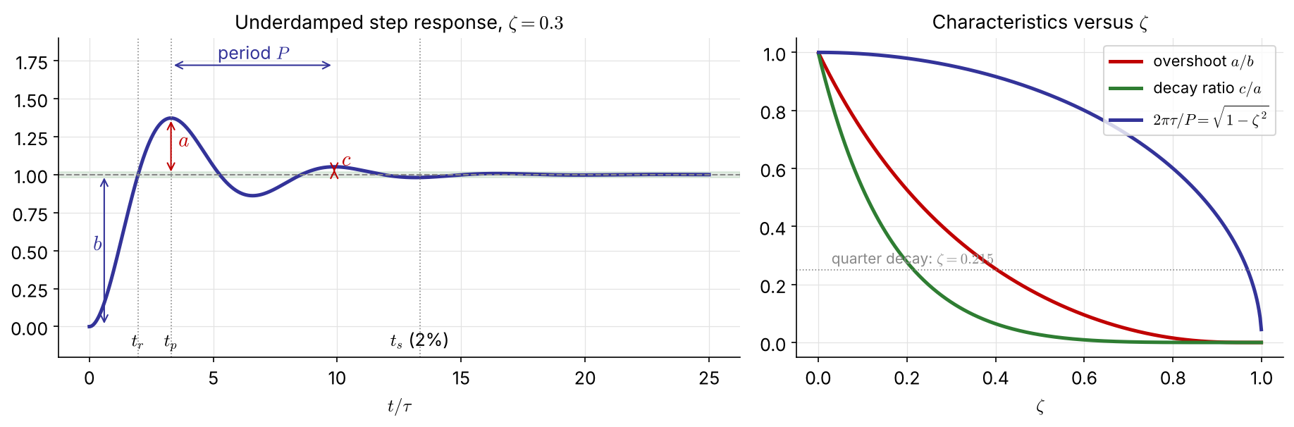
Rarely used directly; the underdamped one yields the characteristics on the next slide.
| overshoot | peak time | rise time | period | settling time | decay ratio |
|---|---|---|---|---|---|
| \(\dfrac ab=\exp\left(\dfrac{-\pi\zeta}{\sqrt{1-\zeta^2}}\right)\) | \(t_p=\dfrac{\pi\tau}{\sqrt{1-\zeta^2}}\) | \(t_r=\dfrac{\tau(\pi-\cos^{-1}\zeta)}{\sqrt{1-\zeta^2}}\) | \(P=\dfrac{2\pi\tau}{\sqrt{1-\zeta^2}}\) | \(t_s\approx\) \(\dfrac{3\tau}{\zeta}\) (5%) \(\dfrac{4\tau}{\zeta}\) (2%) |
\(\dfrac ca=\text{OS}^2\) |
Settling: the envelope \(e^{-\zeta t/\tau}\) behaves like a first-order term with time constant \(\tau/\zeta\). Smaller \(\zeta\): faster rise, larger overshoot, longer settling.
import numpy as np, control as ct, matplotlib.pyplot as plt
t = np.linspace(0, 15, 1501)
for zeta in (0.5, 1.0, 1.5): # s^2 + 2 zeta s + 1 (tau = 1)
G = ct.tf(1, [1, 2*zeta, 1])
plt.plot(t, ct.step_response(G, t).outputs, label=f'zeta = {zeta}')
plt.legend(); plt.xlabel('t')
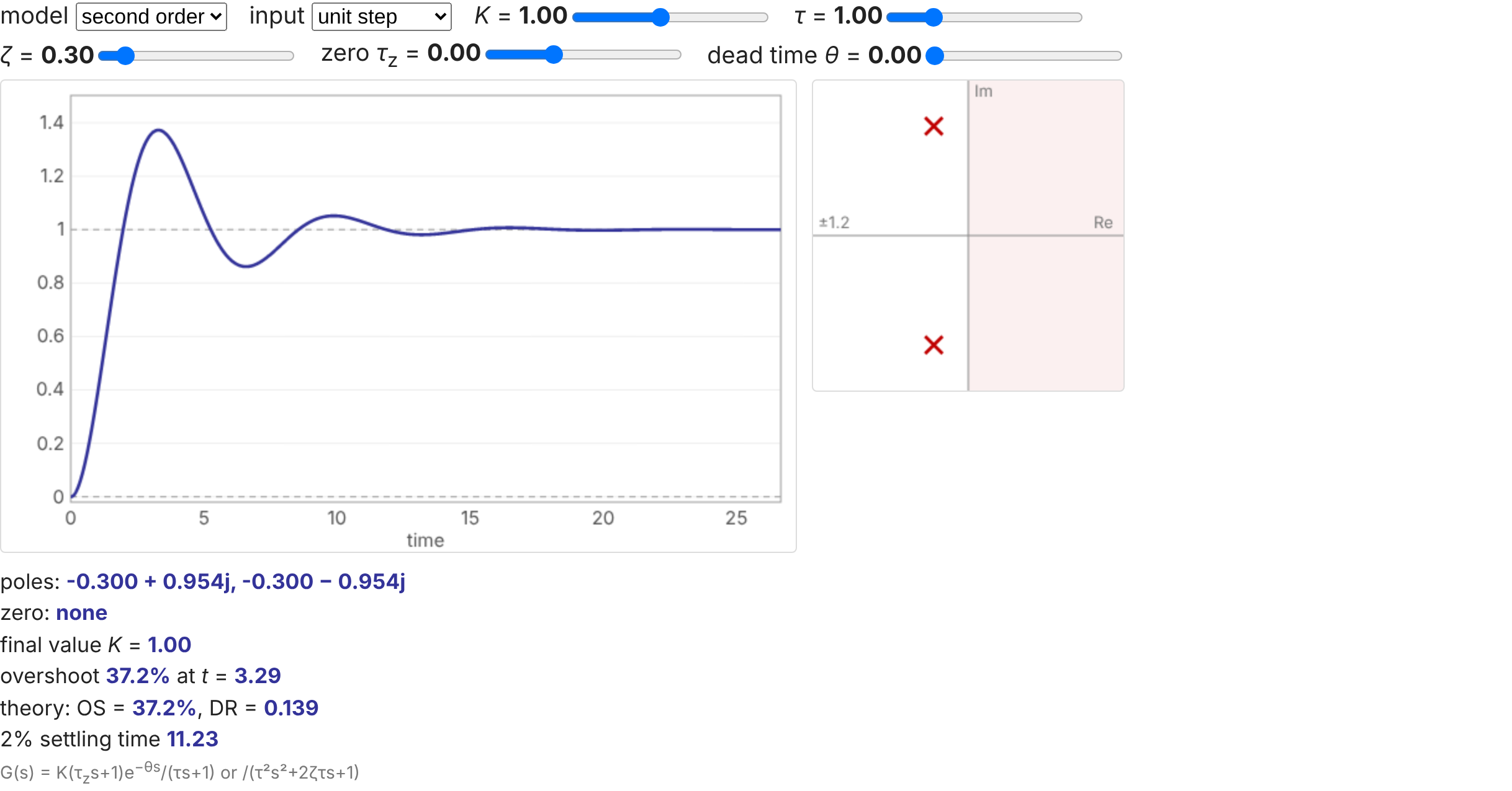
info = ct.step_info(ct.tf(1, [1, 0.6, 1])) # zeta = 0.3
print(info['Overshoot'], info['PeakTime'], info['SettlingTime']) # 37.2 %, 3.29, ...Show that the overdamped step response can be written with two exponentials \(e^{-t/\tau_1}\) and \(e^{-t/\tau_2}\), and find \(\tau_1\), \(\tau_2\) in terms of \(\tau\) and \(\zeta\).
Starting from the underdamped solution, derive the phase-lag form and \(\phi=\tan^{-1}\left(\sqrt{1-\zeta^2}/\zeta\right)\).
Derive the overshoot, peak time, rise time, period and decay ratio in the table.
Caused by fluid travelling down a pipe or a slow analyzer: 시간지연 / 수송지연. \[ y(t)=x(t-t_d)\quad\Rightarrow\quad \frac{Y(s)}{X(s)}=e^{-t_ds} \] \[ \frac{Ke^{-t_ds}}{\tau s+1},\qquad \frac{Ke^{-t_ds}}{\tau^2s^2+2\zeta\tau s+1} \]
Classical tools work with polynomials in \(s\), so we use the Padé approximation, a ratio of polynomials that matches the Taylor series of \(e^{-t_ds}\):
\[ \text{(1/1)}\quad e^{-t_ds}\approx\frac{1-\frac{t_d}2s}{1+\frac{t_d}2s} \] \[ \text{(2/2)}\quad e^{-t_ds}\approx\frac{t_d^2s^2-6t_ds+12}{t_d^2s^2+6t_ds+12} \]
Each adds poles in the LHP and zeros in the RHP, which produce a small initial inverse response instead of a flat delay.
Padé \(P^N_M(x)=\sum_0^Na_nx^n/\sum_0^Mb_nx^n\), \(b_0=1\): the \(N+M+1\) coefficients follow from the Taylor coefficients \(c_n\) by \(a_k=\sum_{j=0}^{k}c_{k-j}b_j\).
\[ \frac{Y}{X}\approx\frac{-1.5s+1}{(10s+1)(1.5s+1)} \]
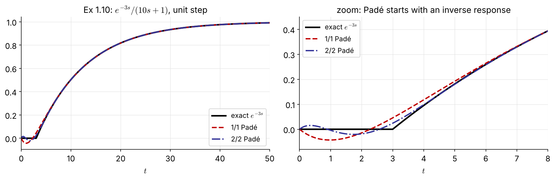
Far from \(t=0\) both approximations are excellent; at early times 1/1 dips to \(-0.04\), and 2/2 wiggles around zero.
Show that the 1/1 Padé approximation is more accurate than the first-order Taylor expansion \(e^{-t_ds}\approx1-t_ds\). (Compare the Taylor series of both.)
Derive the 2/2 Padé approximation and find its poles and zeros for \(t_d=3\).
\(A_i\dfrac{dh_i}{dt}=q_{i-1}-q_i,\ q_i=\dfrac{h_i}{R_i}\) (linear resistance): \[ \frac{H_i(s)}{H_{i-1}(s)}=\frac{K_i}{\tau_is+1},\quad \tau_i=A_iR_i,\ K_i=\frac{R_i}{R_{i-1}} \] \[ \frac{H_n(s)}{Q_1(s)}=\frac{R_n}{(\tau_1s+1)\cdots(\tau_ns+1)} \]
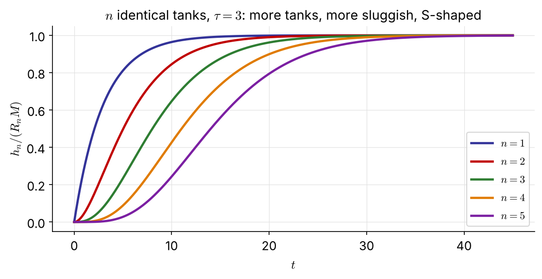
The more tanks, the longer the \(n\)-th tank waits to “see” a change: the response looks like a delay followed by a lag.
Keep the dominant (large) time constants and lump the small ones into a dead time: \[ G(s)\approx\frac{Ke^{-t_ds}}{(\tau_1s+1)(\tau_2s+1)},\quad t_d\approx\sum_{i\ne1,2}\tau_i \]
\[ \frac YX=\frac{3}{(0.1s+1)(0.5s+1)(s+1)(3s+1)} \]
Half rule (Skogestad) NEW: split the largest neglected time constant, half to the lag, half to the delay, e.g. \(\dfrac{3e^{-0.35s}}{(1.25s+1)(3s+1)}\).
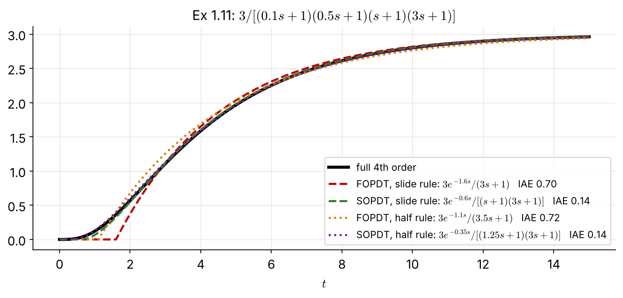
The second-order approximation is clearly better (IAE 0.14 vs 0.70). FOPDT models are the basis of the empirical tuning rules of Ch 3.
\(A_1\dfrac{dh_1}{dt}=q_i-\dfrac{h_1-h_2}{R_1},\quad A_2\dfrac{dh_2}{dt}=\dfrac{h_1-h_2}{R_1}-\dfrac{h_2}{R_2}\) \[ \frac{H_1}{Q_i}=\frac{R_1\tau_2s+R_1+R_2}{p(s)},\qquad \frac{H_2}{Q_i}=\frac{R_2}{p(s)} \] \[ p(s)=\tau_1\tau_2s^2+\left(\tau_1+\tau_2+\tau_1\frac{R_2}{R_1}\right)s+1 \]
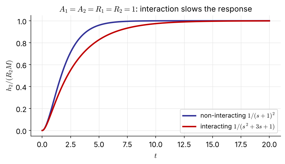
Which damps inlet-flow disturbances better? The interacting pair: the extra term pushes one pole closer to the origin, so the response is slower and smoother. NEW
A nearly perfectly mixed blending tank (first order) feeds a downstream unit through a long transfer pipe. A test shows that the pipe behaves as if its volume were split into five equal perfectly stirred tanks in series.
\(V_{tank}=2\ \text{m}^3,\quad V_{pipe}=0.1\ \text{m}^3,\quad q_{total}=1\ \text{m}^3/\text{min}\)
What is the most accurate transfer function \(C'_{out}(s)/C'_{in}(s)\) you can develop?
What approximate low-order transfer function could represent this process?
What do you conclude about the need to model the pipe’s mixing accurately?
Simulate the approximate and full-order responses to a step change in \(c_{in}\).
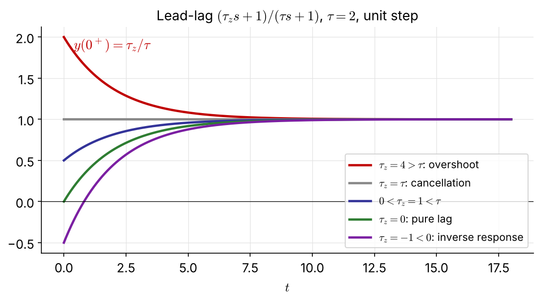
Poles govern the inherent dynamics; zeros add finer “fingerprints” by changing the coefficients. \[ \frac{Y}{X}=\frac{\tau_zs+1}{\tau s+1}\ \xrightarrow{X=1/s}\ Y=\frac1s+\frac{\tau_z-\tau}{\tau s+1} \] \[ y(t)=1-\left(1-\frac{\tau_z}{\tau}\right)e^{-t/\tau},\qquad y(0^+)=\frac{\tau_z}{\tau} \]

Two competing effects with different time constants: \[ \frac{Y}{X}=\frac{K_1}{\tau_1s+1}+\frac{K_2}{\tau_2s+1}=\frac{K(\tau_zs+1)}{(\tau_1s+1)(\tau_2s+1)} \] \(K=K_1+K_2,\quad \tau_z=\dfrac{K_1\tau_2+K_2\tau_1}{K_1+K_2}\)
With opposing effects (\(K_2<0\)), superposition gives a rough picture right away.
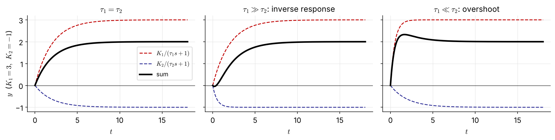
The fast element wins first, the large-gain element wins at the end: \(\tau_1\gg\tau_2\) gives \(\tau_z<0\) and an inverse response.
\[ \frac YX=\frac{K(\tau_zs+1)}{(\tau_1s+1)(\tau_2s+1)},\qquad \tau_1>\tau_2 \]
Calculate the response to a step of magnitude \(M\) and show that

Interactive version: seoultechpse.github.io/ProCon/ch1/ch1_dynamics.html — first or second order, \(K\), \(\tau\), \(\zeta\), zero \(\tau_z\), dead time \(\theta\).

Tools
Responses
Next (Ch 2): close the loop with a controller and see how \(K_c\), \(\tau_I\), \(\tau_D\) move these poles.