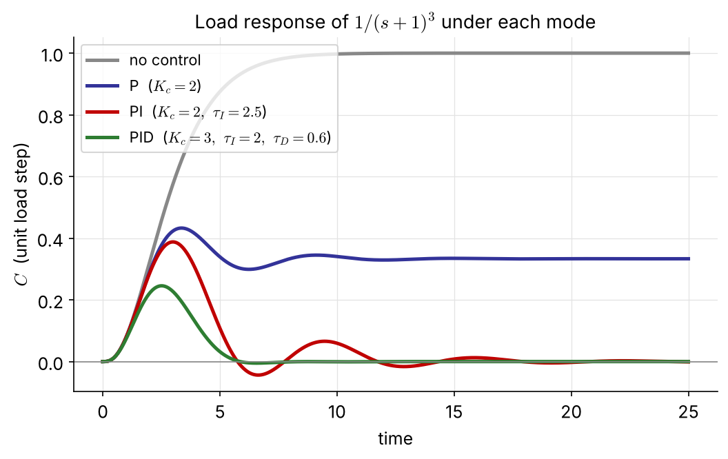
2. Analysis of Single-Loop Control Systems
We finally launch into controllers. Two things come first:
| Section | Topic | Key result |
|---|---|---|
| 2.1 | the feedback loop, block diagrams, hardware | \(C=G_{sp}R+G_{load}L\), characteristic equation \(1+G_{OL}=0\) |
| 2.2 | P, PI, PD and PID control | offset, reset windup, derivative kick |
| 2.3 | closed-loop response, Examples 2.1–2.6 | how \(K_c,\ \tau_I,\ \tau_D\) change gain, time constant and \(\zeta\) |
| 2.4 | which controller for which variable | level, flow, temperature, pressure, composition |
Feedback control is old: water-level regulators in Greece around 250 B.C., James Watt’s fly-ball governor in 1788.
The controller acts on the error, the negative of the deviation:
\[ e(t)=h^s-h(t),\qquad p(t)=p^s+f\big[e(t)\big] \]
\(f\) is the control law; \(p^s\) is the controller bias, the output when \(e=0\).
A system means the process together with the controller and its accessories (sensor, transmitter, actuator).
For negative feedback, \(E=R-HY\) and \(Y=GE\), so \(Y=G(R-HY)\) and
\[ \frac{Y}{R}=\frac{G}{1+GH} \]
Rule. Closed-loop TF \(=\) (product of the blocks on the forward path) \(/\) (1 \(+\) product of all blocks around the loop).
The denominator, set to zero, is the characteristic equation of the closed loop.
Process model \(T=G_LT_i+G_pT_H\). We manipulate the steam temperature \(T_H\) (\(M\)), so the inlet temperature \(T_i\) becomes the load \(L\). Closing the loop:
\[ C=\underbrace{\frac{K_mG_cG_aG_p}{1+G_mG_cG_aG_p}}_{G_{sp}}\,R+\underbrace{\frac{G_L}{1+G_mG_cG_aG_p}}_{G_{load}}\,L \]
\(K_m\) converts the set point (°C) into the same mA signal as the measurement, so \(K_m\) must equal the steady-state gain of \(G_m\). NEW
Servo problem — set-point change, \(L=0\): \[ C=G_{sp}R,\qquad \text{ideal: } C=R \] (perfect tracking)
Regulator problem — disturbance, \(R=0\): \[ C=G_{load}L,\qquad \text{ideal: } C=0 \] (perfect disturbance rejection)
Both transfer functions share one denominator, the closed-loop characteristic equation:
\[ 1+G_mG_cG_aG_p=1+G_{OL}=0 \]
Dynamics and stability are therefore the same for set-point and load changes. Only the numerators, and so the size and shape of the response, differ.
Controlled variables: those that
Manipulated variables: those that
In a SISO system everything else becomes a load variable.
The temperature \(T\) of a tray near the top of a distillation column is controlled by adjusting the reflux flow \(R\). Draw a block diagram for this feedback loop. Treat both the feed flow rate \(F\) and the feed composition \(x_F\) as disturbances.
Hint: two load blocks, \(G_F\) and \(G_{x_F}\), enter the same summing junction as \(G_p\).
Every block has units. Standard signal ranges let instruments from different vendors talk to each other: 4–20 mA for electronic signals (4 mA is the live zero), 3–15 psi for pneumatic valve actuators, with an I/P transducer in between.
\[ G_m=\frac{T_m}{T}=\frac{K_me^{-t_ds}}{\tau_ms+1} \]
Thermowell, energy balance: \[ m_mC_m\frac{dT_m}{dt}=U_mA_m(T-T_m)\ \Rightarrow\ \tau_m=\frac{m_mC_m}{U_mA_m} \]
A fast sensor with no transport lag gives simply \(G_m=K_m\).
Example 20–120 °C is transmitted linearly as 4–20 mA.
\[ I=mT+I_0,\quad m=\frac{16\ \text{mA}}{100\ ^\circ\text{C}}=0.16\ \text{mA}/^\circ\text{C} \] \(I_0=4-20(0.16)=0.8\) mA
The transmitter gain is \[ K_m=\frac{\text{output span}}{\text{input span}}=0.16\ \text{mA}/^\circ\text{C} \]

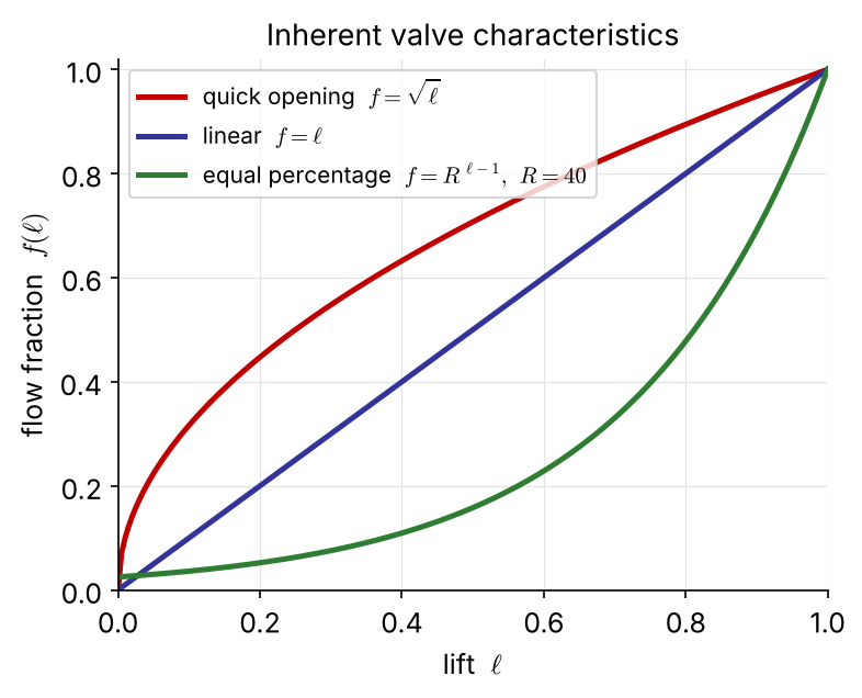
\[ q=C_vf(\ell)\sqrt{\frac{\Delta P_v}{g_s}} \]
\(C_v\): valve coefficient, \(\ell\): lift (0–1), \(f(\ell)\): valve characteristic.
The actuator must cover the range of the manipulated variable and respond faster than the process.
Fail-safe action NEW: air-to-open (fail closed) or air-to-close (fail open), chosen for safety when the air supply fails. It fixes the sign of the valve gain.
Lumping I/P, valve and steam coil: \[ G_a=G_v=\frac{K_v}{\tau_vs+1},\quad K_v=0.6\ ^\circ\text{C/mA},\ \tau_v=0.2\ \text{min} \]

\[ G_p=\frac{0.85}{20s+1},\quad G_v=\frac{0.6}{0.2s+1} \]
\(G_m=K_m=0.16\) mA/°C (the transmitter above).
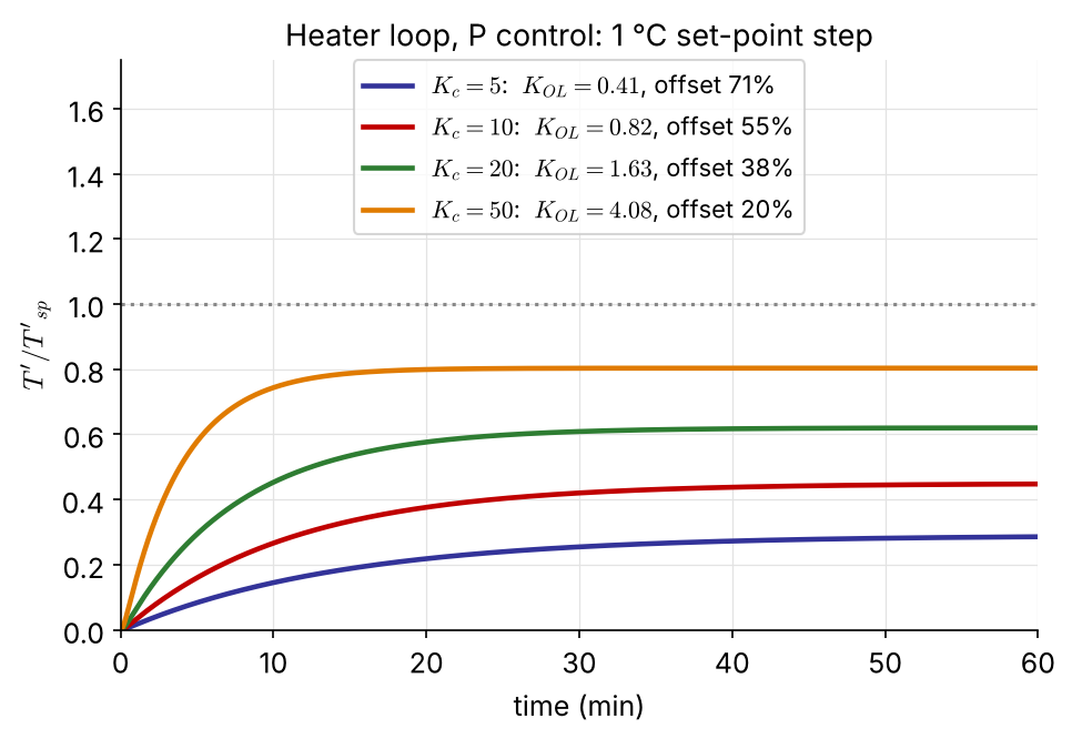
With P control, \(G_c=K_c\) (mA/mA): \[ K_{OL}=K_cK_vK_pK_m=0.0816\,K_c \] \[ \text{offset}=\frac{1}{1+K_{OL}} \]
The loop gain is the product of all the gains, so a sluggish transmitter or valve gain must be made up by \(K_c\). P control alone always leaves an offset, which motivates integral action.
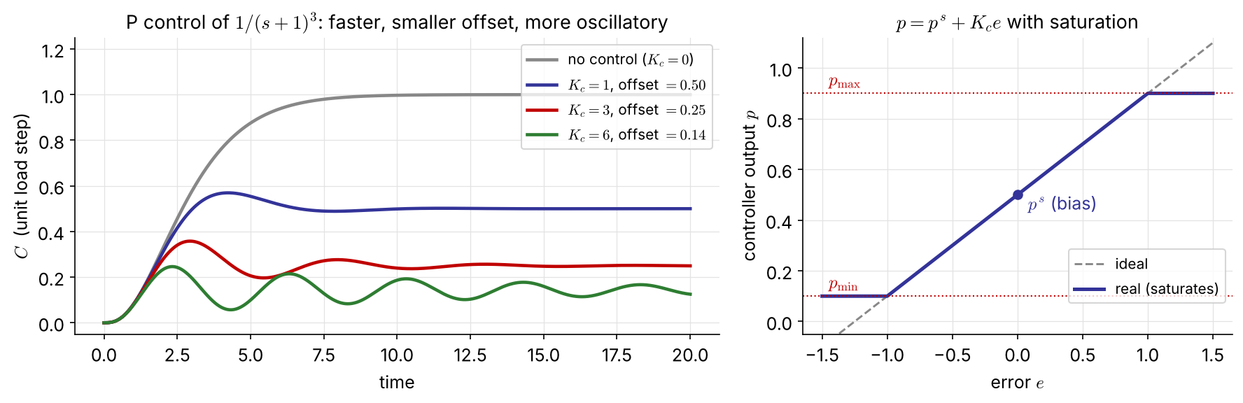
\[ p(t)=p^s+K_ce(t)\ \Rightarrow\ G_c(s)=\frac{P(s)}{E(s)}=K_c \] (in deviation variables, \(e^s=0\))
Action: NEW reverse acting (\(K_c>0\)): output falls as the measurement rises. Direct acting (\(K_c<0\)) is needed when the process gain is negative, so that \(K_cK_p>0\).
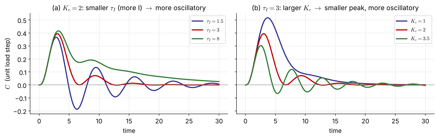
\[ p(t)=p^s+K_c\left[e(t)+\frac{1}{\tau_I}\int_0^te\,dt\right]\ \Rightarrow\ G_c(s)=K_c\left[1+\frac{1}{\tau_Is}\right] \]
\(\tau_I\): integral (reset) time; \(1/\tau_I\) is the reset rate. Integral action is never used alone. The integral keeps changing as long as \(e\ne0\), so it can supply the new output that a steady state needs while \(e=0\): no offset.
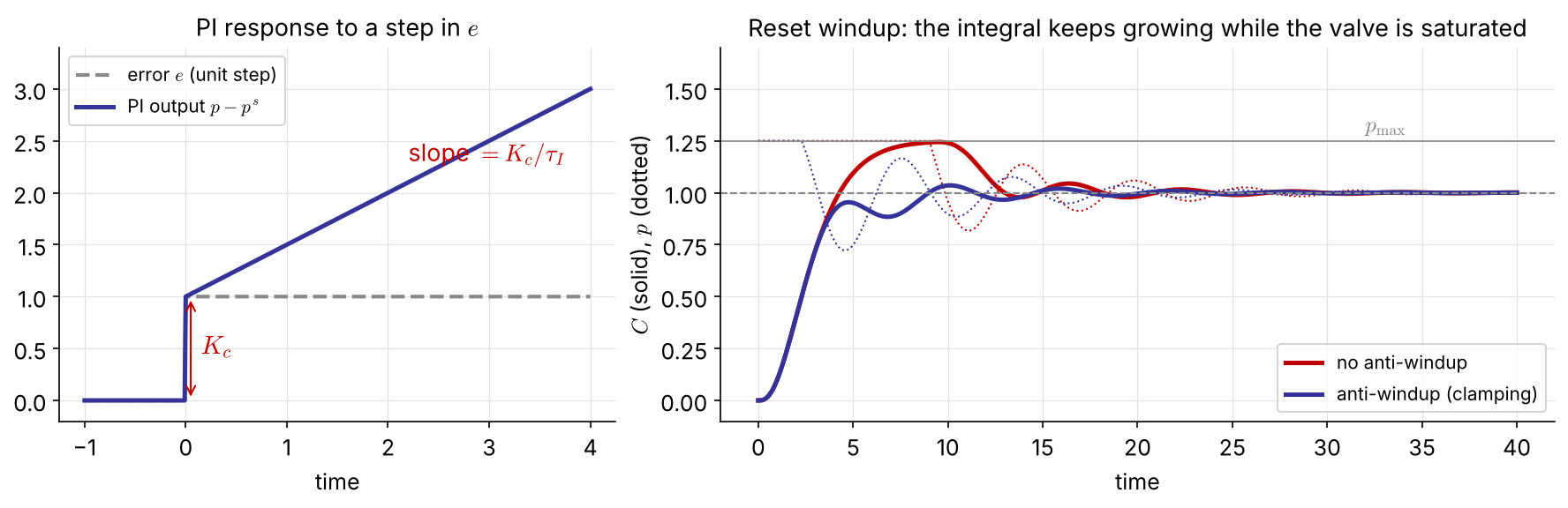
Reset windup: when \(e\) persists (start-up, large set-point changes) the integral grows until the valve saturates, then must “unwind”, which causes a long overshoot. Anti-windup stops integrating while the output is saturated.
\[ p(t)=p^s+K_c\left[e+\tau_D\frac{de}{dt}\right]\ \Rightarrow\ G_c=K_c[1+\tau_Ds] \]
Ideal derivative action cannot be built (more zeros than poles), so a lead-lag element is used: \[ G_c=K_c\frac{\tau_Ds+1}{\alpha\tau_Ds+1},\qquad 0.05\le\alpha\le0.2 \]
This adds a fast pole at \(s=-1/(\alpha\tau_D)\) that limits the high-frequency gain to \(K_c/\alpha\).
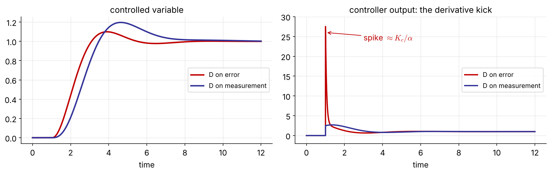
A set-point step makes \(de/dt\) infinite, and the filtered D produces a spike of about \(K_c/\alpha\) in the controller output.
Acting on the measurement instead of the error removes it: \(R\) reaches the output only through the PI part. For a load change (\(R\) constant) nothing changes, since then \(de/dt=-dC/dt\).
| Form | \(G_c(s)\) | Where |
|---|---|---|
| ideal (ISA) | \(K_c\left[1+\dfrac{1}{\tau_Is}+\tau_Ds\right]=K_c\dfrac{\tau_I\tau_Ds^2+\tau_Is+1}{\tau_Is}\) | analysis |
| parallel | \(K_c+\dfrac{K_I}{s}+K_Ds\), \(K_I=\dfrac{K_c}{\tau_I},\ K_D=K_c\tau_D\) | Simulink, textbooks |
| real (filtered D) | \(K_c\left[1+\dfrac{1}{\tau_Is}+\dfrac{\tau_Ds}{\alpha\tau_Ds+1}\right]\) | most industrial controllers |
| series (interacting) | \(K_c\left[\dfrac{\tau_Is+1}{\tau_Is}\right]\left[\dfrac{\tau_Ds+1}{\alpha\tau_Ds+1}\right]\) | pneumatic, older analog |

| P | I | D | |
|---|---|---|---|
| speed | ↑ | ↑ | – |
| offset | ↓ but stays | removed | – |
| overshoot | ↑ | ↑ | ↓ |
| stability margin | ↓ | ↓ | ↑ (usually) |
| noise sensitivity | – | – | ↑ |
Arrows: effect of increasing \(K_c\), \(1/\tau_I\) and \(\tau_D\). NEW
Start simple: P, then PI; add D only if it helps.
Proportional-only control of the stirred-tank heater above. The transmitter has a span of 50 °F and a zero of 55 °F. Nominal conditions are \(\bar T=80\) °F and \(\bar T_i=65\) °F. \(K_c=5\), \(K_v=1.2\) (dimensionless), \(K_{IP}=0.75\) psi/mA, \(\tau=5\) min; valve and transmitter dynamics are negligible. After the set point is changed from 80 to 85 °F, the tank temperature settles at 84.14 °F.
(a) What is the offset? (b) What is the process gain \(K_2\)? (c) What is the pressure signal \(p_t\) to the valve at the final steady state?
\[ \frac{C}{R}=\frac{G_cG_p}{1+G_cG_p} \]
\(G_m=G_a=1\) and \(L=0\) keep the algebra light. The ideas carry over to the full loop.
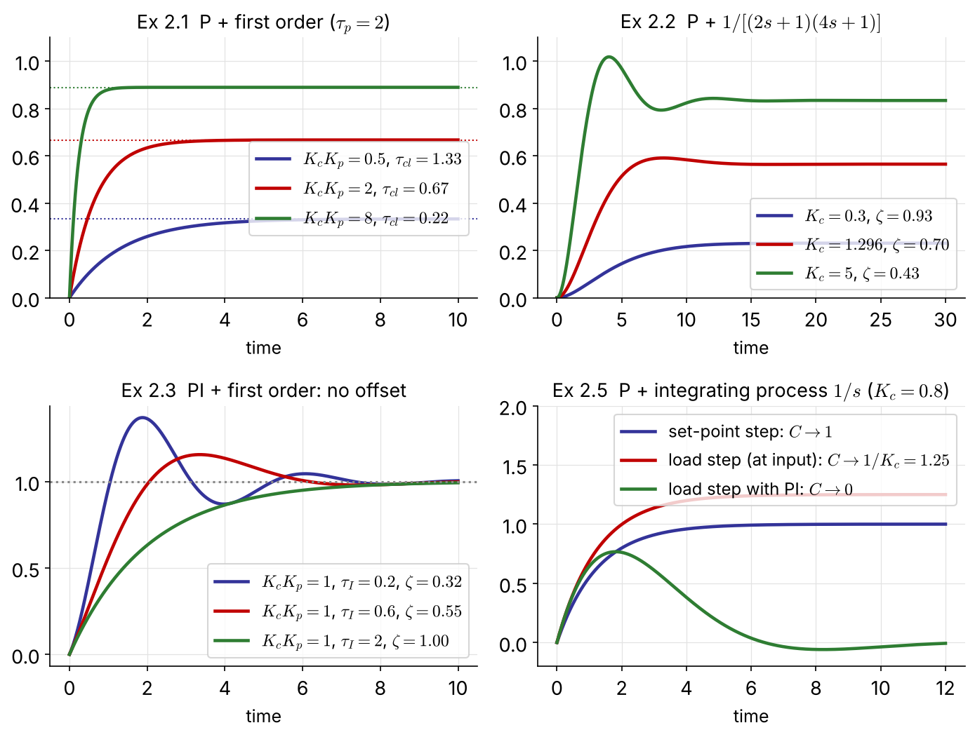
\(G_c=K_c,\quad G_p=\dfrac{K_p}{\tau_ps+1}\) What is \(C(\infty)\) after a unit set-point step?
\[ \frac{C}{R}=\frac{K_cK_p}{\tau_ps+1+K_cK_p}=\frac{K_{cl}}{\tau_{cl}s+1},\qquad K_{cl}=\frac{K_cK_p}{1+K_cK_p},\quad \tau_{cl}=\frac{\tau_p}{1+K_cK_p} \]
Larger \(K_c\) shrinks both \(\tau_{cl}\) and the offset, but the offset vanishes only as \(K_c\to\infty\).
A first-order process under P control cannot oscillate or go unstable for \(K_cK_p>0\); real loops do because of the lags and dead time this model ignores.
\(G_p=\dfrac{K_p}{(\tau_1s+1)(\tau_2s+1)}\), \(\;\tau_1=2,\ \tau_2=4\) min, \(K_p=1\). Which \(K_c\) gives \(\zeta=0.7\)?
\[ \frac{C}{R}=\frac{K_cK_p}{\tau_1\tau_2s^2+(\tau_1+\tau_2)s+1+K_cK_p}=\frac{K_{cl}}{\tau^2s^2+2\zeta\tau s+1} \]
\[ \tau=\sqrt{\frac{\tau_1\tau_2}{1+K_cK_p}},\qquad \zeta=\frac{\tau_1+\tau_2}{2\sqrt{\tau_1\tau_2(1+K_cK_p)}} \]
\(\zeta=\dfrac{3}{\sqrt{8(1+K_c)}}=0.7\ \Rightarrow\ 1+K_c=2.296\)
\(K_c=1.30\), offset \(=\dfrac{1}{1+K_c}=0.44\): large!
Raising \(K_c\) lowers \(\zeta\): the closed loop becomes underdamped although the open loop is overdamped. Speed and damping trade off, and the offset at \(\zeta=0.7\) is unacceptable.
\(G_c=K_c\left(1+\dfrac{1}{\tau_Is}\right)\), \(\;G_p=\dfrac{K_p}{\tau_ps+1}\). What is the offset?
\[ \frac{C}{R}=\frac{K_cK_p(\tau_Is+1)}{\tau_I\tau_ps^2+\tau_I(1+K_cK_p)s+K_cK_p}=\frac{\tau_Is+1}{\tau^2s^2+2\zeta\tau s+1} \]
\[ \tau=\sqrt{\frac{\tau_I\tau_p}{K_cK_p}},\qquad \zeta=\frac12(1+K_cK_p)\sqrt{\frac{\tau_I}{K_cK_p\tau_p}} \]
\(\lim_{s\to0}C/R=1\): no offset.
The integrator raises the order by one: a first-order process can now oscillate (small \(\tau_I\), large \(K_c\)).
The closed loop also has a zero at \(s=-1/\tau_I\), which adds overshoot beyond what \(\zeta\) alone predicts.
\(G_c=K_c(1+\tau_Ds)\), \(\;G_p=\dfrac{K_p}{\tau_ps+1}\)
\[ \frac{C}{R}=\frac{K_cK_p(\tau_Ds+1)}{(\tau_p+K_cK_p\tau_D)s+1+K_cK_p} =K_{cl}\,\frac{\tau_Ds+1}{\tau_{cl}s+1} \]
\[ K_{cl}=\frac{K_cK_p}{1+K_cK_p},\qquad \tau_{cl}=\frac{\tau_p+K_cK_p\tau_D}{1+K_cK_p} \]
The ideal D makes \(C\) jump at \(t=0^+\) to \(K_{cl}\tau_D/\tau_{cl}\). On a first-order process derivative action brings little; it pays off on higher-order processes, where it adds damping.
\(G_c=K_c\), \(\;G_p=\dfrac{K_p}{s}\) (e.g. a level with a pumped outlet). What is the offset?
Servo \[ \frac{C}{R}=\frac{K_cK_p}{s+K_cK_p}=\frac{1}{\tau s+1},\ \ \tau=\frac{1}{K_cK_p} \]
\(C(\infty)=1\): no offset for set-point changes. The process already contains an integrator.
Regulator NEW (load at the process input, \(G_L=G_p\)) \[ \frac{C}{L}=\frac{K_p}{s+K_cK_p}\ \Rightarrow\ C(\infty)=\frac{1}{K_c} \]
A step disturbance still leaves an offset. Only an integrator in the controller (PI) removes it.

| Ex | \(G_c\) | \(G_p\) | CL order | offset |
|---|---|---|---|---|
| 2.1 | P | 1st | 1 | \(\dfrac{1}{1+K_cK_p}\) |
| 2.2 | P | 2nd | 2 | \(\dfrac{1}{1+K_cK_p}\) |
| 2.3 | PI | 1st | 2 | 0 |
| 2.4 | PD | 1st | 1 | \(\dfrac{1}{1+K_cK_p}\) |
| 2.5 | P | \(K_p/s\) | 1 | 0 (servo) |
Offset disappears only when the loop contains an integrator between the error and the disturbance.
import numpy as np, control as ct
import matplotlib.pyplot as plt
Gp = ct.tf(0.8, [5, 1])
t = np.linspace(0, 6, 601)
Gc = 10 # P
Gcl = ct.feedback(Gp*Gc, 1) # 8/9
plt.plot(t, ct.step_response(Gcl, t).outputs)
Gc = ct.tf([10, 10], [1, 0]) # PI
Gcl = ct.feedback(Gp*Gc, 1)
plt.plot(t, ct.step_response(Gcl, t).outputs)
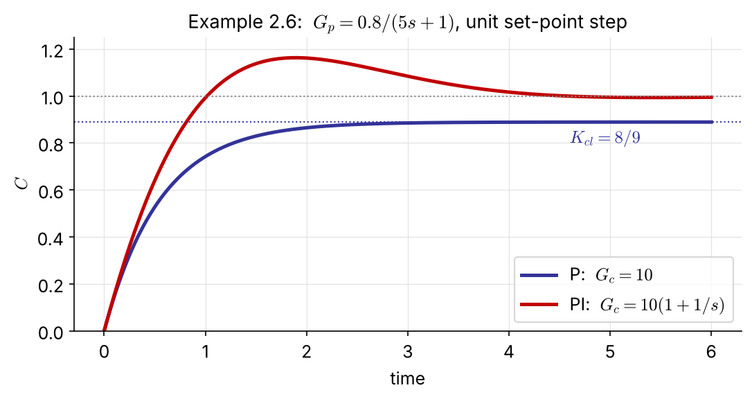
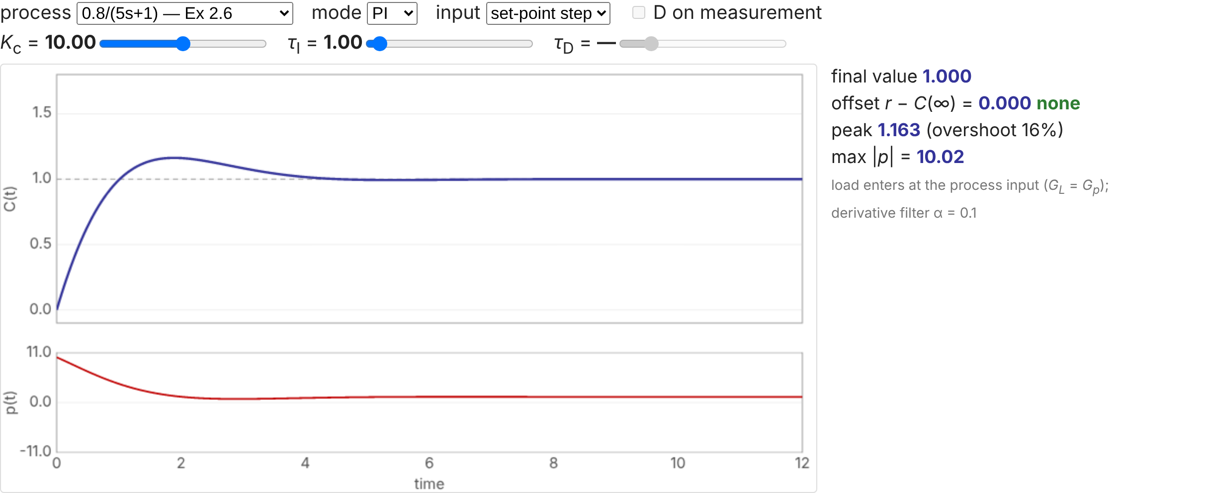
P: \(K_{cl}=8/9\), offset 0.11. PI: no offset, \(\zeta=0.71\), 16% overshoot. In Simulink the same loop is a Step, a Sum, two gains with an integrator (PI) and a Transfer Fcn block.

Interactive version: seoultechpse.github.io/ProCon/ch2/ch2_analysis.html — process, mode, \(K_c\), \(\tau_I\), \(\tau_D\), set-point or load step.

| Variable | Usual choice | Why |
|---|---|---|
| level | P | only needs to stay within a range around the set point |
| flow | PI | fast, noisy loop: low to moderate \(K_c\), small \(\tau_I\) for fast tracking |
| temperature | PID | heat-transfer lags make it sluggish; offsets are rarely acceptable; PI alone is slow |
| pressure, flash-drum vapor | PI | fast and tight, like flow control |
| pressure, column top (via condenser cooling) | P, or PID if speed matters | slow heat-exchanger dynamics rule out PI |
| composition, fast analyzer (pH, UV/IR) | PI or PID | decide from the process dynamics |
| composition, slow analyzer (GC) | sampled-data control | large measurement delay |
Know the hardware (actuators, sensors) from handbooks and manuals. Prevalent time delay is what makes chemical process control harder than many mechanical or electrical systems.
The exit concentration \(c_3\) is controlled with stream 2.
(a) Draw the block diagram of the composition loop. (b) Derive each transfer function and substitute numbers. (c) The PI controller was tuned at the nominal conditions. Should it be retuned when (i) \(\bar c_2\) changes to 8.5 lb/ft³; (ii) the transmitter span becomes 3–14 lb/ft³; (iii) its zero is moved so that it reads 4–10 lb/ft³? Justify briefly.
| \(p_t\) (psi) | 6 | 9 | 12 |
|---|---|---|---|
| \(q_2\) (gal/min) | 20 | 15 | 10 |
Setting up
PID modes
Next (Ch 3): how to choose \(K_c\), \(\tau_I\) and \(\tau_D\). Then (Ch 4–5): when the loop goes unstable.