A differential equation (DE) is an equation containing the derivatives of one or more dependent variables with respect to one or more independent variables
An \(n\)-th order ODE, \(F\left( x, y, y', \cdots, y^{(n)} \right) = 0\), \(\,\)is linear in the variable \(y\,\) if \(\,F\) is linear in \(y, y',\cdots,y^{(n)}\)
An ODE is nonlinear if
The coefficients of \(y, y',\cdots,y^{(n)}\) contain the dependent variable \(y\) or its derivatives
Powers of \(y, y',\cdots,y^{(n)}\) appear in the equation or
Nonlinear functions of the dependent variable or its derivatives (e.g., \(\sin y\) or \(e^{y'}\)) appear in the equation
1.1.4 Solution of an ODE
Any function \(\phi\), defined on an interval \(I\) and possessing at least \(n\) derivatives that are continuous on \(I\), which when substituted into an ODE reduces the equation to an identity, is a solution
Interval \(I\) can be an open interval \((a,b)\), a closed interval \([a,b]\), an infinite interval \((a,\infty)\), etc.
A solution of a differential equation that is identically zero on an interval \(I\) is a trivial solution
The graph of a solution \(\phi\) of an ODE is a solution curve and it is continuous on its interval \(I\) while the domain of \(\phi\) may differ from the interval \(I\)
An explicit solution is one in which the dependent variable is expressed solely in terms of the independent variable and constants
\(G(x,y)=0\,\) is an implicit solution, if at least one function \(\phi\) exists, that satisfies the relation \(G\) and the ODE on \(I\)
1.1.5 Families of Solutions
Similar to integration, we obtain a solution to a first-order differential equation containing an arbitrary constant \(c\)
A solution with a constant \(c\) represents a set \(G(x,y,c)=0\) of solutions, called a one-parameter family of solutions
An \(n\)-parameter family of solutions \[ G(x,y,c_1,c_2,\cdots,c_n)=0 \]
solves an \(n\)-th order differential equation
1.1.6 Systems of Differential Equations
Two or more equations involving the derivatives of two or more unknown functions of a single independent variable are called the system of differential equations
When solving an IVP, consider whether a solution exists and whether the solution is unique
Existence:\(\,\) Does the differential equation possess solutions and do any of the solution curves pass through the initial point \((x_0, y_0)\)?
Uniqueness:\(\,\) When can we be certain there is precisely one solution curve passing through the initial point \((x_0, y_0)\)?
Theorem 1.1 gives conditions that are sufficient to guarantee the existence and uniqueness of a solution \(y(x)\) to a first-order IVP
\(f(x,y)\) and \(\displaystyle\frac{\partial f}{\partial y}\) are continuous on the region \(\,R\,\) for the interval \(\,I_0\)
Example\(\,\) First-order IVP
\(y(x)=ce^x\) is a one-parameter family of solutions of the first-order DE \(~y'=y\)
Find a solution of the first-order IVP with initial condition \(y(0)=3\)
Solution
From the initial condition, we obtain \(3=ce^0\)
Solving, we find \(c=3\)
The solution of the IVP is \(y=3e^x\)
Example\(\,\) Second-order IVP
\(x(t) = c_1 \cos 4t +c_2 \sin 4t\)\(\,\)is a two-parameter family of solutions of the second-order DE \(~x''+16x=0\)
Find a solution of the second-order IVP with initial conditions \(~x\left( \frac{\pi}{2} \right) =-2, \;x'\left (\frac{\pi}{2} \right)=1\)
Solution
Substituting for initial conditions and solving for constants, we find \(c_1=-2\) and \(c_2=1/4\)
The solution of the IVP is \(~x(t)=-2\cos 4t +\frac{1}{4}\sin 4t\)
1.3 Differential Equations as Mathematical Models
A mathematical model is a description of a system or a phenomenon
Differential equation models are used to describe behavior in various fields
Biology
Chemistry
Physics
Steps of the modeling process
Example\(\,\) Radioactive Decay
In modeling the phenomenon, it is assumed that the rate \(\displaystyle\frac{dA}{dt}\) at which the nuclei of a substance decays is proportional to the amount \(A(t)\) remaining at time \(t\) given an initial amount of radioactive substance on hand \(A_0\)
\[\frac{dA}{dt} = -kA, \;A(0)=A_0\]
This differential equation also describes a first-order chemical reaction
Example\(\,\) Draining Tank
Toricelli’s law states that the exit speed \(v\) of water through a sharp-edged hole at the bottom of a tank filled to a depth \(h\) is the same as the speed it would acquire falling from a height \(h\), \(\,\)\(v=\sqrt{2gh}\)
Volume \(V\) leaving the tank per second is proportional to the area of the hole \(A_h\)\[\frac{dV}{dt}=-A_h\sqrt{2gh}\]
The volume in the tank at \(t\)\(\,\)is\(\,\)\(V(t)=A_w h\), \(\,\) in which \(\,\)\(A_w\) is the constant area of the upper water surface
Combining expressions gives the differential equation for the height of water at time \(t\)\[\frac{dh}{dt}=-\frac{A_h}{A_w}\sqrt{2gh}\]
Worked Exercises
1.2: 1.\(~y=1/(1 +c_1 e^{-x})\) is a one-parameter family of solutions of the first-order DE \(y'=y -y^2\). \(\,\) Find a solution of the first-order IVP consisting of this differential equation and the given initial condition:
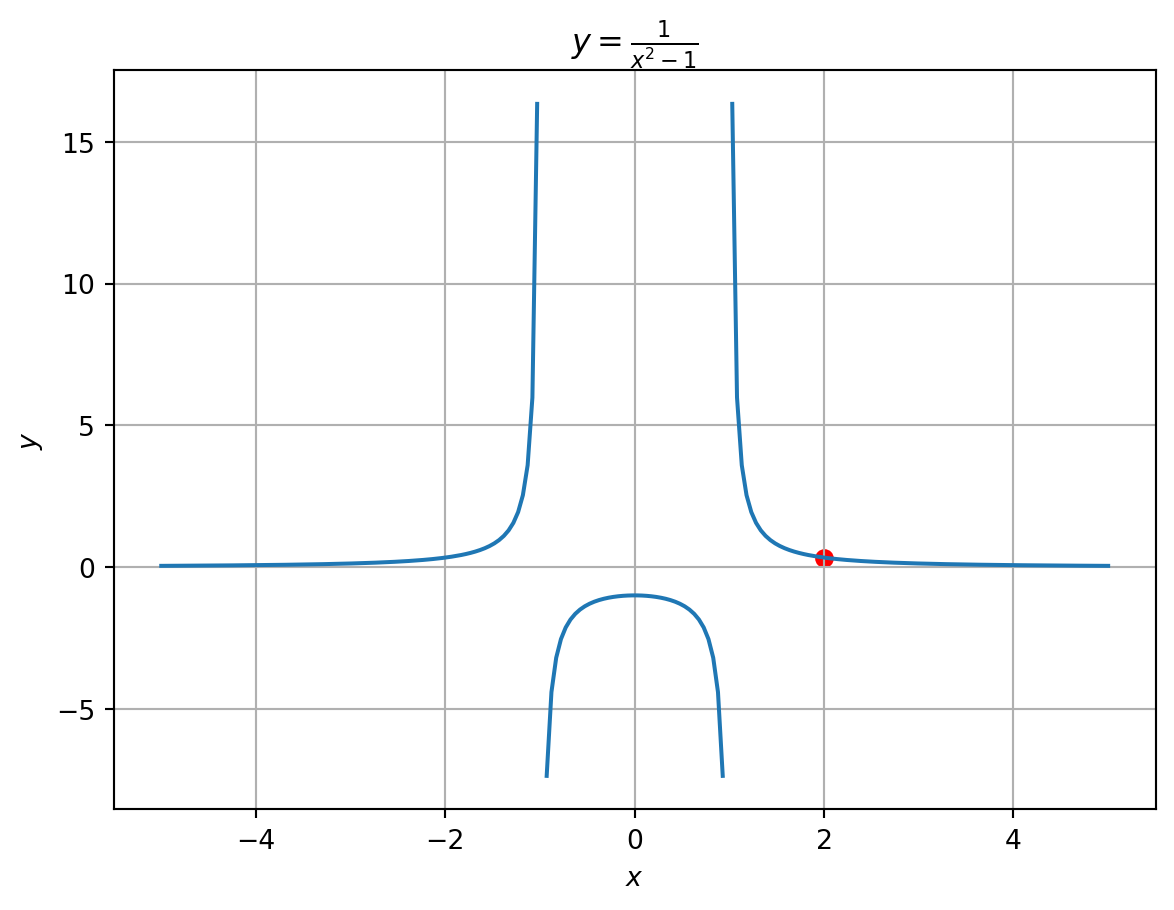
1.2: 3.\(~y=1/(x^2 +c)\) is a one-parameter family of solutions of the first-order DE \(y' +2xy^2=0\). Find a solution of the first-order IVP consisting of this differential equation and the given initial condition. Give the largest interval \(I\) over which the solution is defined
\[y(2)=\frac{1}{3}\]
Solution
\[
\begin{aligned}
y &= \frac{1}{x^2 +c}\\
&\Downarrow {\scriptstyle \text{at } x = 2}\\
\frac{1}{3} &= \frac{1}{4 +c} \\
&\Downarrow \\
c = -1 \, &, \;\; I =(1,\infty) \\
&\Downarrow \\
y &= \frac{1}{x^2 -1}
\end{aligned}\]
1.2: 7.\(\,x(t)=c_1\cos t +c_2\sin t\) is a two-parameter family of solutions of the second-order DE \(x''+x=0\). Find a solution of the second-order IVP consisting of this differential equation and the given initial conditions
\[x(0)=-1, \; x'(0)=8\]
Solution
\[
\begin{aligned}
x(t) &= c_1\cos t +c_2\sin t \\
&\Downarrow \;{\scriptstyle x(0)=-1, \; x'(0)=8}\\
-1 &= c_1 \\
8 &= c_2 \\
&\Downarrow \\
x(t) &= -\cos t +8\sin t
\end{aligned}\]
1.2: 17.\(\,\) Determine a region of the xy-plane for which the given differential equation would have a unique solution whose graph passes through a point \((x_0, y_0)\) in the region.
\[\frac{dy}{dx}=y^{2/3}\]
Solution
Step 1:\(~\)Identify the Function and Its Partial Derivative
Let:
\[f(x, y) = y^{2/3}\]
Then the partial derivative with respect to \(y\) is:
\(f(x, y) = y^{2/3}\) is continuous for all real values of \(x\) and \(y\)
However, \(\frac{\partial f}{\partial y} = \frac{2}{3} y^{-1/3}\) is undefined at \(y = 0\), since \(y^{-1/3}\) is not defined at \(y = 0\)
Step 3:\(~\)Apply the Existence and Uniqueness Theorem
The Existence and Uniqueness Theorem requires both \(f(x, y)\) and \(\frac{\partial f}{\partial y}\) to be continuous in a neighborhood of the initial point \((x_0, y_0)\)
So, a unique solution exists through \((x_0, y_0)\) only if \(y_0 \ne 0\)
By inspection, find a one-parameter family of solutions of the differential equation \(xy'=y\). Verify that each member of the family is a solution of the initial value problem \(xy'=y, \,y(0)=0\)
Explain part 1. by determining a region \(R\) in the \(xy\)-plane for which the differential equation \(xy'=y\) would have a unique solution through a point \((x_0, y_0)\) in \(R\)
Verify that the piecewise-defined function
\[y= \begin{cases}
0, & x < 0 \\
x, & x \ge 0
\end{cases}\]
satisfies the condition \(y(0)=0\). Determine whether this function is also a solution of the initial-value problem in part 1
Solution
Step 1:\(~\)Solve by Inspection
Let’s try separating variables or guessing solutions:
Given: \[xy’ = y \quad \Rightarrow \quad y’ = \frac{y}{x}\]
This is separable:
\[\frac{dy}{y} = \frac{dx}{x}\]
Integrate both sides:
\[\ln |y| = \ln |x| + C_1\]
Exponentiate:
\[|y| = C_2|x| \quad \Rightarrow \quad y = Cx\]
for some constant \(C \in \mathbb{R}\), because the sign of \(C_2\) absorbs the absolute values. So the one-parameter family of solutions is:
\[y = Cx\]
Step 2:\(~\)Verify with the Initial Condition
We are given the initial value problem:
\[xy’ = y, \quad y(0) = 0\]
Let’s plug \(x = 0\) into the general solution:
\[y = Cx \Rightarrow y(0) = C \cdot 0 = 0\]
So for any value of \(C\), the condition \(y(0) = 0\) is satisfied.
❗ But Wait – What About Uniqueness?
Let’s look back at the original differential equation:
\[y’ = \frac{y}{x}\]
This function \(f(x, y) = \frac{y}{x}\) is not defined at \(x = 0\), so the existence and uniqueness theorem does not apply at \(x = 0\)
That means:
Infinitely many solutions of the form \(y = Cx\) pass through \((0, 0)\),
But there is no unique solution to the initial value problem,
So although each \(y = Cx\) satisfies both the differential equation and the initial condition, the IVP does not have a unique solution
\(~\)
1.3: 5.\(\,\) A cup of coffee cools according to Newton’s law of cooling. Use data from the graph of the temperature \(T(t)\) in figure to estimate the constants \(T_m\), \(T_0\), and \(k\) in a model of the form of the first-order initial-value problem
\[ \frac{dT}{dt}=k(T -T_m), \;\;T(0)=T_0 \]
Solution
\[
\begin{aligned}
\frac{dT}{dt} &=k(T -T_m), \;\;T(0)=T_0 \\
&\Downarrow \\
T(0) &= T_0 \\
T(\infty) &= T_m \\
\ln \left( \frac{T -T_m}{T_0 -T_m} \right) &= k t \\
&\Downarrow \\
k \text{ is the slope of the graph of }\, & t \text{ vs. } \ln \left( \frac{T -T_m}{T_0 -T_m}\right)
\end{aligned}\]
1.3: 19. After a mass \(m\) is attached to a spring, it stretches \(s\) units and then hangs at rest in the equilibrium position as shown in Figure (b). After the spring/mass system has been set in motion, let \(x(t)\) denote the directed distance of the mass beyond the equilibrium position. As indicated in Figure (c), assume that the downward direction is positive, that the motion takes place in a vertical straight line through the center of gravitiy of the mass, and that the only forces acting on the system are the weight of the mass and the restoring force of the stretched spring. Use Hooke’s law: The restoring force of a spring is proportional to its total elongation. Determine a differential equation for the displacement \(x(t)\) a time \(t\)
Solution
To model the vertical motion of a spring-mass system as described, we need to:
Use Newton’s Second Law: \(~F = ma\),
Use Hooke’s Law: The restoring force is proportional to the total elongation of the spring,
Let \(y(t)\) denote the displacement from equilibrium (positive downward),
Assume only gravity and the spring’s restoring force act
Step 1:\(~\)Define the Forces
Let:
\(m =\) mass (kg),
\(g =\) acceleration due to gravity (m/s²),
\(k =\) spring constant (N/m),
\(y(t) =\) displacement from equilibrium (m), with positive direction downward
From equilibrium condition:
When the mass is at rest (before any motion), gravity is balanced by the spring force:
\[mg = k \Delta l \quad \text{(equilibrium stretch)}\]
Step 2:\(~\)After the System is Set in Motion
When displaced by \(y(t)\) from equilibrium:
Weight (constant force downward): \(~F_g = mg\)
Spring force (upward restoring force): \(~F_s = -k(\Delta l + y)\)
But since we’re measuring \(y(t)\) from equilibrium, the net restoring force becomes:
\[F_{\text{net}} = -k y(t)\]
Thus, from Newton’s second law:
\[m \ddot{y}(t) = -k y(t)\]
Step 3:\(~\)Final Differential Equation
\[m \ddot{y} + k y = 0\]
This is a second-order linear differential equation that governs the vertical motion of the mass from equilibrium