When \(\mathbf{r}\) have continuous first derivative and \(\mathbf{r}'(t)\neq\mathbf{0}~\) for all \(~t~\) in the open interval \((a,b),\)\(\,\)then \(\mathbf{r}\) is said to be a smooth function
In the case of the second derivative, \(\,\)we have
If \(\mathbf{r}\) is a differentiable vector function and \(s=u(t)\) is a differentiable scalar function, then the derivative of \(\mathbf{r}(s)\) with respect to \(t\) is
If \(~\mathbf{r}(t) = f(t)\mathbf{i} +g(t)\mathbf{j} +h(t)\mathbf{k}\,\) is a smooth function, \(\,\)then it can be shown that the length of the smooth curve traced by \(\,\mathbf{r}\,\) is given by
Thus, \(\displaystyle\,\frac{d\mathbf{v}}{dt} \cdot \mathbf{v}=0\)\(\text{ }\)or\(\text{ }\)\(\mathbf{a}(t) \cdot \mathbf{v}(t)=0~\,\) for all \(\,t\)
Centripetal Acceleration
For circular motion in the plane, described by \(\mathbf{r}(t) = r_0 \cos\omega t \,\mathbf{i} +r_0\sin\omega t \,\mathbf{j},\)\(\,\)it is evident that
\[\mathbf{r}''=-\omega^2\mathbf{r}\]
This means that the acceleration vector \(\mathbf{a}(t)=\mathbf{r}''(t)\) points in the direction opposite to that of the position vector \(\mathbf{r}(t)\). \(\,\) We then say \(~\mathbf{a}(t)\) is centripetal acceleration
10.3 Curvature and Components of Acceleration
We know that \(\mathbf{r}'(t)\) is a tangent vector to the curve \(C\), and consequently
\[
\begin{aligned}
\frac{d\mathbf{r}}{dt} &=\frac{d\mathbf{r}}{ds}
\frac{ds}{dt}\;\text{ and so }\\[5pt]
\frac{d\mathbf{r}}{ds} =
\frac{\displaystyle\frac{d\mathbf{r}}{dt}} {\displaystyle\frac{ds}{dt}}
&=\frac{\mathbf{r}'(t)}{\left\| \mathbf{r}'(t) \right\|}
= \mathbf{T}(t)
\end{aligned}\]
Let \(\,\mathbf{r}(t)\,\) be a vector function defining a smooth curve \(C\). \(\,\)If \(s\) is the arc length parameter and \(\mathbf{T}\) is the unit tangent vector, \(\,\)then the curvature of \(C\) at a point is
In other words, \(\,\)curvature is given by \(\,\kappa(t)=\frac{\displaystyle\left\|\mathbf{T}'(t)\right\|}{\displaystyle\left\|\mathbf{r}'(t)\right\|}\)
Tangential and Normal Components of Acceleration
The velocity of the particle on \(C\) is \(~\mathbf{v}(t)=\mathbf{r}'(t)\), \(\,\)whereas its speed is \(\displaystyle\frac{ds}{dt}=v=\| \mathbf{v}(t) \|\). \(\,\) Thus, \[\mathbf{v}(t)=v\mathbf{T}\]
Differentiating this last expression with respect to \(t\) gives acceleration
It follows from the differentiation of \(\mathbf{T}\cdot\mathbf{T}=1\,\) that \(\displaystyle\,\mathbf{T}\cdot \frac{d\mathbf{T}}{dt}=0\). \(\,\)If \(\displaystyle\,\left\|\frac{d\mathbf{T}}{dt}\right\| \neq 0\), \(\,\)the vector
is a unit normal to the curve \(C\). \(\,\)The vector \(\mathbf{N}\) is also called the principal normal
Since curvature is \(\displaystyle\,\kappa = \frac{\left\|\frac{d\mathbf{T}}{dt} \right\|}{v}\), \(\,\) it follows that \(\displaystyle\frac{d\mathbf{T}}{dt}=\kappa v \mathbf{N}\). \(\,\)Thus
If \(z=f(u,v)\) is differentiable and \(u=g(t)\,\) and \(v=h(t)\) are differentiable functions of a single variable \(t\), \(\,\)the ordinary derivative \(\displaystyle\frac{dz}{dt}\) is
The gradient vector \(\nabla f\) points in the direction in which \(f\) increases most rapidly, \(\,\)whereas \(-\nabla f\) points in the direction of the most decrease of \(\,f\)
\(~\)
10.6 Tangent Planes and Normal Lines
\(\nabla f\) is orthogonal to the level curve at \(P\)
The derivative of \(\,f\left(x(t), \,y(t)\right)=c\,\) with respect to \(\,t\,\) is
Stated another way, \(\,\)if \(C_1\) and \(C_2\) are two different paths between the same points \(A\) and \(B\), \(\,\)then we expect that \[\int_{C_1} \mathbf{F}\cdot \,d\mathbf{r} \neq \int_{C_2} \mathbf{F}\cdot \,d\mathbf{r}\]
Path Independence
A line integral \(\displaystyle\int_C \mathbf{f}\cdot d\mathbf{r}~\) is independence of the path if
for any two paths \(C_1\) and \(C_2\) between \(A\) and \(B\)
A vector function \(\mathbf{f}\) in 2- or 3-space is said to be conservative if \(\,\mathbf{f}\) can be written as the gradient of a scalar function \(\phi\). \(\,\)The function \(\phi\) is called a potential function for \(\,\mathbf{f}\)
In other words, \(\,\mathbf{f}\) is conservative if there exists a function \(\phi\) such that \(\,\mathbf{f}=\nabla \phi\). \(\,\)A conservative vector field is also called a gradient vector field
Fundamental Theorem
If \(~\mathbf{f}(x,y,z)~\) is a conservative vector field in \(R\) and \(\phi\) is a potential function for \(\,\mathbf{f}\), \(\,\)then
is a conservative vector field in an open region of 3-space, and that \(P\), \(Q\), and \(R\) are continuous and have continuous first partial derivatives in that region
Then \(\,\mathbf{f}=\nabla \phi\,\) and \(\,\nabla\times\mathbf{f}=\nabla\times\nabla\phi=\mathbf{0}\), \(\,\)that is
Suppose that \(C\) is a piecewise-smooth simple closed curve bounding a simply connected region \(R\)
If \(\,P\), \(Q\), \(\displaystyle\frac{\partial P}{\partial y}\), and \(\displaystyle\frac{\partial Q}{\partial x}\) are continuous on \(R\), \(\,\)then
\[
\begin{aligned}
\iint_R &\left( \frac{\partial Q}{\partial x} -\frac{\partial P}{\partial y} \right)\, dA \\
&=\iint_{R_1} \left( \frac{\partial Q}{\partial x} -\frac{\partial P}{\partial y} \right)\, dA
+\iint_{R_2} \left( \frac{\partial Q}{\partial x} -\frac{\partial P}{\partial y} \right)\, dA\\
&=\oint_{C_1} P \,dx +Q \,dy +\oint_{C_2} P \,dx +Q \,dy =\oint_C P \,dx +Q \,dy
\end{aligned}\]
\(~\)
Example\(\,\) Evaluate \(\displaystyle\oint_{C} \frac{-y}{x^2 +y^2}\, dx + \frac{x}{x^2 + y^2}\,dy\), \(\,\) where \(C=C_1 \cup C_2\) is the boundary of the shaded region \(R\)
\[
\begin{aligned}
\mathbf{u} &= \Delta x_k \mathbf{i} +f_x(x_k,y_k)\Delta x_k \mathbf{k}\\
\mathbf{v} &= \Delta y_k \mathbf{j} +f_y(x_k,y_k)\Delta y_k \mathbf{k}\\
& \Downarrow \\
\mathbf{u} \times \mathbf{v} &={\scriptsize\left[-f_x(x_k,y_k)\mathbf{i} -f_y(x_k,y_k)\mathbf{j}+\mathbf{k}\right] \Delta x_k \Delta y_k}\\
& \Downarrow \\
\Delta S_k &= {\sqrt{1 +\left[\,f_x(x_k,y_k)\right]^2 +\left[\,f_y(x_k,y_k)\right]^2}\Delta A_k }
\end{aligned}\] Then the area of the surface over \(R\) is given by \[ { S=\iint_R \sqrt{1+\left[\,f_x(x,y)\right]^2 +\left[\,f_y(x,y)\right]^2}\,dA} \]
Surface Integral
Let \(\,G\,\) be a function of three variables defined over a region of space containing the surface \(S\). \(\,\)Then the surface integral of \(G\) over \(S\) is given by
Let \(S\) be a piecewise-smooth orientable surface bounded by a piecewise-smooth simple closed curve \(C\)
Let \(~\mathbf{f}(x,y,z)=P(x,y,z)\mathbf{i} +Q(x,y,z)\mathbf{j} +R(x,y,z)\mathbf{k} \,\) be a vector field for which \(P\), \(Q\), and \(R\) are continuous and have continuous first partial derivatives in a region of 3-space containing \(S\). \(~\)If \(C\) is traversed in the positive direction, then
where \(\displaystyle\,\mathbf{n}=\frac{dy}{ds}\mathbf{i} -\frac{dx}{ds}\mathbf{j}\)
Divergence Theorem
Let \(D\,\) be a closed and bounded region in 3-space with a piecewise-smooth boundary \(S\) that is oriented outward
Let \(\;\mathbf{f}(x,y,z)=P(x,y,z)\,\mathbf{i}+Q(x,y,z)\,\mathbf{j} +R(x,y,z)\,\mathbf{k}~\) be a vector field for which \(P\), \(Q,\) and \(R\) are continuous first partial derivatives in a region of 3-space containing \(D\). \(\,\) Then
2.\(~\) Find an equation of the plane containing \((1, 7, -1)\) that is perpendicular to the line of intersection of \(-x +y -8z=4~\) and \(~3x -y +2z=0\)
Solution
Step 1:\(~\) Find direction vector of the line of intersection
The line of intersection of two planes lies in both planes, and its direction vector is perpendicular to both normals of the planes
So, compute the cross product of the normal vectors of the two planes
Normal to \(\pi_1\): \(~\mathbf{n}_1 = \langle -1, 1, -8 \rangle\)
Normal to \(\pi_2\): \(~\mathbf{n}_2 = \langle 3, -1, 2 \rangle\)
4.\(~\) Find the work done by the given force \(~\mathbf{f}=(x-y)\mathbf{i} +(x+y)\mathbf{j}~\) around the closed curve in the following
Solution
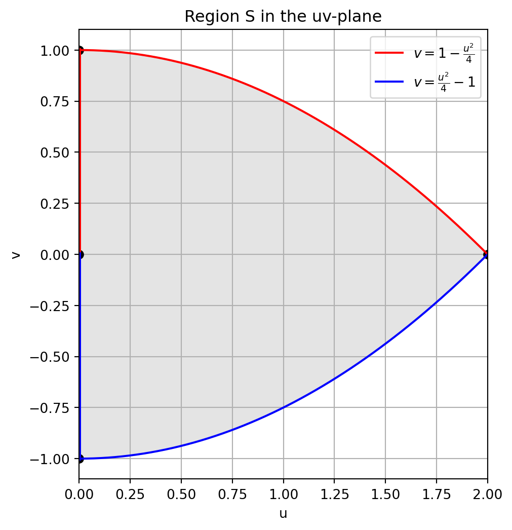
The image shows a region bounded between two quarter circles:
Outer curve: \(x^2 + y^2 = 4\) (radius 2)
Inner curve: \(x^2 + y^2 = 1\) (radius 1)
The region is the quarter annulus in the first quadrant, swept from the positive \(x\)-axis to the positive \(y\)-axis, and the curve is oriented counterclockwise, forming a positively oriented closed curve \(C\)
So \(v = 1\) is the upper limit (since \(v > 0\)), and the region \(S\) is bounded by:
\(0 \le v \le 1\)
\(v \le u \le \frac{2}{1 + v}\)
Step 4:\(~\) Change of variables in the integral
We rewrite the integral in terms of \(u\), \(v\):
\[\iint_S \frac{1}{\sqrt{(u + v +1)^2}} \cdot |J| \, du\, dv\]
So the integrand becomes simply 1. Then the integral becomes the area of the region \(S\):
\[\iint_S 1 \, du\, dv = \int_{v=0}^{1} \int_{u=v}^{\frac{2}{1 + v}} 1 \, du\, dv = \int_0^1 \left( \frac{2}{1 + v} - v \right) dv =2 \ln 2 - \frac{1}{2}\]
\(~\)
6.\(~\) Evaluate the integral
\[ \iint_R (x^2 +y^2) \sqrt[3]{x^2 -y^2} \,dA \]
where \(R\) is the region bounded by the graphs of \(x=0\), \(x=1\), \(y=0\), and \(y=1\) by means of the change of variables \(u=2xy\), \(v=x^2 -y^2\)
Solution
Step 1:\(~\) Compute the Jacobian
We need the Jacobian determinant \(J = \left| \frac{\partial(x, y)}{\partial(u, v)} \right|\), but we are given \(u = 2xy\), \(v = x^2 - y^2\), so we compute \(\frac{\partial(u, v)}{\partial(x, y)}\) and then take the reciprocal for the change of variables
12.\(~\) Let a particle of mass \(m\) travel along a differentiable path \(\mathbf{x}\) in a Newtonian vector field \(\mathbf{F}\) (i.e., one that satisfies Newton’s second law \(\mathbf{F} = m\mathbf{a}\), where \(\mathbf{a}\) is the acceleration of \(\mathbf{x}\)). We define the angular momentum\(\mathbf{l}(t)\) of the particle to be the cross product of the position vector and the linear momentum \(m\mathbf{v}\), i.e.,
\[\mathbf{l}(t) = \mathbf{x}(t) \times m \mathbf{v}(t)\]
(Here \(\mathbf{v}\) denotes the velocity of \(\mathbf{x}\).) The torque about the origin of the coordinate system due to the force \(\mathbf{F}\) is the cross product of position and force:
Thus, we see that the rate of change of angular momentum is equal to the torque imparted to the particle by the vector field \(\mathbf{F}\)
\((b)\) Suppose that \(\mathbf{F}\) is a central force (i.e., a force that always points directly towards or away from the origin). Show that in this case the angular momentum is conserved, that is, that it must remain constant
Using \(1-\cos t=2\sin^2(t/2)\), \(~\) this becomes the simpler form
\[\kappa(t)=\frac{1}{4a\,|\sin(t/2)|}\]
At \(t=\pi\), \(~\sin(\pi/2)=1\), so
\[\boxed{\kappa(\pi)=\frac{1}{4a}}\]
\(~\)
14.\(~\) Find the osculating plane to the following circular helix at \(t=\pi/4\)
\[\mathbf{r}(t) = -2 \sin t \mathbf{i} +2\cos t\mathbf{j} +3 t\mathbf{k}\]
\(~\)
Solution
For \(\mathbf r(t)=\left<-2\sin t,\,2\cos t,\,3t \right>\), the osculating plane at \(t_0\) is the plane through \(\mathbf r(t_0)\) whose normal is the binormal vector \[\mathbf B(t_0)=\frac{\mathbf r’(t_0)\times\mathbf r’’(t_0)}{\|\mathbf r’(t_0)\times\mathbf r’’(t_0)\|}\]
At \(t=\pi/4\): \[\mathbf r\!\left(\tfrac{\pi}{4}\right)=\big(-\sqrt2,\;\sqrt2,\;\frac{3\pi}{4}\big)\] and \[\mathbf r’\!\left(\tfrac{\pi}{4}\right)\times\mathbf r’’\!\left(\tfrac{\pi}{4}\right)
= \begin{pmatrix}3\sqrt2\\[4pt]3\sqrt2\\[4pt]4\end{pmatrix}\]
Use this cross product as the plane normal. The osculating plane equation is \[(3\sqrt2,\,3\sqrt2,,\,4)\cdot\big((x,y,z)-(-\sqrt2,\sqrt2,\frac{3\pi}{4})\big)=0\] Expanding and simplifying gives the tidy form \[\boxed{\,3\sqrt2 (x+y) +4z=3\pi\,}\] which is the osculating plane at \(t=\pi/4\)
\(~\)
15.\(~\) Let \(\boldsymbol{\omega} = \nabla \times \mathbf{u}\) represent the vorticity of an inviscid, barotropic fluid governed by the Euler equation
\[\frac{D\mathbf{u}}{Dt} =-\frac{1}{\rho}\nabla p + \mathbf{f}\]
where \(\frac{D}{Dt}\) denotes the material derivative (\(\frac{\partial}{\partial t}+\mathbf{u} \cdot \nabla\)). Under the barotropic assumption, the pressure is a function of density alone, \(p = p(\rho)\)
(a) Take the curl of the Euler equation to obtain the evolution equation for the vorticity field
(b) Show that for an inviscid, barotropic fluid with conservative body forces, \[\Gamma(t)=\oint_{C(t)} \mathbf{u} \cdot d\mathbf{r}\] remains constant in time if \(C(t)\) moves with the fluid. Hint Differentiate \(\Gamma(t)\): \[\frac{d\Gamma}{dt}=\oint_{C(t)}\frac{D\mathbf{u}}{Dt} \cdot d\mathbf{r}\]
(c) Evaluate \(\frac{D\omega_z}{Dt}\) for a two-dimensional incompressible flow, and discuss the resulting consequences for the evolution of vortex patches and vortex sheets
Solution
(a)Curl the Euler equation \(\rightarrow\) vorticity evolution
Euler (compressible) in material-derivative form:
\[\frac{\partial \mathbf u}{\partial t}+(\mathbf u\cdot\nabla)\mathbf u
= -\frac{1}{\rho}\nabla p+\mathbf f\]
Define vorticity \(\boldsymbol\omega=\nabla\times\mathbf u\). Take \(\nabla\times(\cdot)\) of both sides. Use the identity
Differentiate following the moving loop (hint given):
\[\frac{d\Gamma}{dt}=\oint_{C(t)}\frac{D\mathbf u}{Dt}\cdot d\mathbf r
=\oint_{C(t)}\Big(-\frac{1}{\rho}\nabla p+\mathbf f\Big)\cdot d\mathbf r\]
Under barotropic \(p=p(\rho)\) there exists a scalar \(H(\rho)\) (specific enthalpy) with \(\nabla H=\frac{1}{\rho}\nabla p\). If the body force is conservative, \(\mathbf f=-\nabla\Phi\) for some potential \(\Phi\). Then the integrand is a gradient:
\[-\frac{1}{\rho}\nabla p+\mathbf f = -\nabla H -\nabla\Phi = -\nabla(H+\Phi)\]
and the line integral of a gradient around a closed curve vanishes. Hence
\[\frac{d\Gamma}{dt}=0\]
So circulation around any material loop \(C(t)\) is constant in time — this is Kelvin’s circulation theorem (for inviscid, barotropic fluid with conservative body forces)
(c)Two-dimensional incompressible flow:\(\dfrac{D\omega_z}{Dt}\) and consequences
For 2D flow in the \(xy\)-plane, let \(\mathbf u=(u(x,y,t),v(x,y,t),0)\) and assume no \(z\)-dependence. The vorticity has only a \(z\)-component:
For incompressible flow \(\nabla\cdot\mathbf u=0\). Also \((\boldsymbol\omega\cdot\nabla)\mathbf u\) vanishes because \(\boldsymbol\omega\) points in \(z\) and there is no \(z\)-variation:
If body forces are irrotational so \(\nabla\times\mathbf f=0\), the vorticity equation reduces to
\[\frac{D\omega_z}{Dt}=0\]
So in 2D incompressible Euler flow the scalar vorticity \(\omega_z\) is materially conserved along particle paths
Consequences:
Vortex patches. A vortex patch is a region where \(\omega_z\) is nonzero (often constant) and zero outside. Because \(\omega_z\) is advected with the flow, every fluid particle keeps its initial vorticity value. Thus a patch’s vorticity value is preserved and the patch is merely carried/deformed by the flow. Incompressibility preserves area, so the area of the patch remains constant (though its shape can become complex — e.g. filamentation)
Vortex sheets. A vortex sheet is a curve across which the tangential velocity is discontinuous (equivalently a delta-distribution vorticity concentrated on a curve). In 2D inviscid flow the sheet strength (the jump in tangential velocity, or equivalently circulation per unit length) is transported with the sheet — the sheet is convected by the flow. However, vortex sheets in inviscid flow are nonlinearly unstable (Kelvin–Helmholtz instability) and tend to roll up into spirals (the sheet can develop finer and finer structure). In the ideal Euler limit this leads to complicated, potentially singular behavior; with even small viscosity the sheet diffuses and rolls up more smoothly
No vortex stretching in 2D. Because there is no \((\boldsymbol\omega\cdot\nabla)\mathbf u\) term, vorticity cannot be amplified by stretching as it can in 3D. This is the fundamental reason 2D turbulence and vortex dynamics differ qualitatively from 3D: vorticity values are conserved along particle paths, and inverse energy cascade / persistence of coherent vortices are characteristic features
\(~\)
16. Let \(\mathbf{u}(x,y,z)=\left<-y f(r,z),\ x f(r,z),\ g(r,z)\right>,\quad r=\sqrt{x^2+y^2}\)
(a) In cylindrical coordinates \((r,\theta,z)\), find the condition from \(\nabla\cdot\mathbf{u}=0\)
(b) Assuming no \(\theta\)-dependence, show that there exists a streamfunction \(\Psi(r,z)\) such that \[u_r=\frac{1}{r}\frac{\partial\Psi}{\partial z},\qquad
u_z=-\frac{1}{r}\frac{\partial\Psi}{\partial r}\]
(c) Write the formal decomposition \(\mathbf{u}=\nabla\phi+\nabla\times\mathbf{A}\). Discuss what \(\phi\) (and boundary conditions on \(\mathbf{A}\), this part is optional) become for incompressible flow
(d) For \(f(r,z)=\dfrac{\alpha}{(r^2+z^2)^{3/2}}\), \(g=0\), compute \(\boldsymbol{\omega}=\nabla\times\mathbf{u}\) and describe its physical meaning
Solution
Throughout use cylindrical coordinates \((r,\theta,z)\) with \[x=r\cos\theta,\qquad y=r\sin\theta\] and unit vectors \[\mathbf e_r=(\cos\theta,\sin\theta,0),\;\mathbf e_\theta=(-\sin\theta,\cos\theta,0),\;\mathbf e_z=(0,0,1)\]
A quick and useful observation from the given Cartesian form \[\mathbf u=(-y f(r,z),\;x f(r,z),\;g(r,z))\] is that \[u_r=\mathbf u\cdot\mathbf e_r=0,\qquad
u_\theta=\mathbf u\cdot\mathbf e_\theta = r\,f(r,z),\qquad
u_z=g(r,z)\]
(a)Divergence-free condition in cylindrical coordinates
(b)Existence of an axisymmetric stream function \(\Psi(r,z)\)
Assume no \(\theta\)-dependence (axisymmetric). For general axisymmetric flows (not necessarily the special form above) the divergence-free condition becomes
This is the 2D divergence-free condition in the \((r,z)\)-plane for the vector \((r u_r,\; r u_z)\); hence there exists a stream function \(\Psi(r,z)\) (unique up to additive constant) such
\[r u_r=\frac{\partial\Psi}{\partial z},\qquad
r u_z=-\frac{\partial\Psi}{\partial r}\]
Dividing by \(r\) gives the standard axisymmetric Stokes stream function relations
(c)Helmholtz decomposition \(\mathbf u=\nabla\phi+\nabla\times\mathbf A\) and consequences for incompressible flow
The Helmholtz decomposition states any sufficiently smooth vector field on \(\mathbb R^3\) (with suitable decay or boundary conditions) can be written as
\[ \mathbf u=\nabla\phi+\nabla\times\mathbf A \]
where \(\phi\) is a scalar potential and \(\mathbf A\) a vector potential. Taking divergence gives
since \(\nabla\cdot(\nabla\times\mathbf A)=0\). Thus for an incompressible flow \(\nabla\cdot\mathbf u=0\) we have
\[\boxed{\;\nabla^2\phi=0\;}\]
so \(\phi\) is harmonic. With common boundary/decay conditions (e.g. \(\mathbf u\) vanishes at infinity or normal velocity specified on a closed boundary), the only physically allowable harmonic \(\phi\) compatible with zero net flux is typically a constant (so \(\nabla\phi=0\)), and all motion is described by the solenoidal part \(\nabla\times\mathbf A\). In short:
For incompressible flow, \(\phi\) is harmonic; if boundary/decay conditions force \(\phi\) to be constant, the flow is purely solenoidal \(\mathbf u=\nabla\times\mathbf A\)
A convenient gauge for \(\mathbf A\) is the Coulomb gauge \(\nabla\cdot\mathbf A=0\). Then
For incompressible flows with \(\phi\) chosen zero, \(\mathbf A\) solves the vector Poisson equation
\[-\nabla^2\mathbf A=\mathbf u\]
with boundary conditions on \(\mathbf A\) chosen to make the solution unique, e.g. \(\mathbf A\to0\) at infinity and \(\nabla\cdot\mathbf A=0\)
So physically: for incompressible flows the irrotational part is absent (or trivial) under typical no-flux/decay conditions, and the velocity is given entirely by the curl of a vector potential which encodes the vorticity
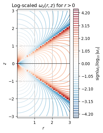
(d)Vorticity for \(f(r,z)=\dfrac{\alpha}{(r^2+z^2)^{3/2}}\), \(g=0\). Physical interpretation
With the specified \(f\) and \(g=0\) the flow is purely azimuthal:
\[u_r=0,\qquad u_\theta = r f(r,z)=\frac{\alpha r}{(r^2+z^2)^{3/2}},\qquad u_z=0\]
Compute the vorticity \(\boldsymbol\omega=\nabla\times\mathbf u.\) For axisymmetric, \(\theta\)-independent fields the cylindrical-component formulas simplify to
The vorticity has no azimuthal component (\(\omega_\theta=0\)); it is in the meridional (poloidal) plane \((r,z)\). Thus swirling motion \(u_\theta\) produces poloidal vorticity — typical of axisymmetric swirling flows
The vorticity field is singular at the origin (behaves like a power of distance) and decays rapidly for large distance: the denominator \((r^2+z^2)^{5/2}\) gives a far-field decay like \(O(\text{distance}^{-5})\) for components (so the induced velocity decays more slowly)
The structure of \(\boldsymbol\omega\) resembles a dipole-like poloidal vorticity: \(\omega_r\) is odd in \(z\) (changes sign across the \(z=0\) plane), while \(\omega_z\) has a quadrupolar character (combination of \(r^2\) and \(z^2\)). Vorticity lines (integral curves of \(\boldsymbol\omega\)) lie in meridional planes and encircle/loop around the symmetry axis — qualitatively similar to a vortex ring/poloidal-dipole structure concentrated near the origin
Physically this flow can be seen as an idealized concentrated swirl (azimuthal velocity decaying like \((\text{distance})^{-2}\) for large distance because \(u_\theta\sim r/(r^2+z^2)^{3/2}\)), and the computed \(\boldsymbol\omega\) describes the local twisting/rotation of fluid elements produced by that swirl. The sign pattern indicates opposite vorticity above and below the midplane \(z=0\) in the radial component, etc
import numpy as npimport matplotlib.pyplot as pltimport matplotlib.colors as colorsalpha =1.0# Grid for r > 0 regionr = np.linspace(0.02, 3, 100)z = np.linspace(-3, 3, 80)R, Z = np.meshgrid(r, z)# Define vorticity component ω_zs = R**2+Z**2omega_z = alpha *(-R**2+2*Z**2) /s**(2.5)# Compute log10 of magnitude and preserve signlog_omega = np.sign(omega_z) * np.log10(np.abs(omega_z) +1e-10)# --- Plot log-scaled ω_z ---plt.figure(figsize=(3, 5))cont = plt.contour(R, Z, log_omega, levels=60, cmap="RdBu_r")plt.colorbar(cont, label=r"$\mathrm{sign}(\omega_z)\log_{10}|\omega_z|$")plt.title(r"Log-scaled $\omega_z(r,z)$ for $r > 0$")plt.xlabel("$r$")plt.ylabel("$z$")plt.axhline(0, color='k', lw=0.8)plt.grid(True)plt.axis("equal")plt.show()