import numpy as np
import matplotlib.pyplot as plt
from matplotlib import animation, rc
from IPython.display import HTML

plt.rcParams['font.size'] = 12
plt.rcParams['xtick.direction'] = 'in'
plt.rcParams['ytick.direction'] = 'in'13 Hyperbolic Partial Differential Equations
13.1 The One-dimensional Wave Equation
We will now begin to study the second major class of PDEs, \(\,\)hyperbolic equations
Vibrating-String Problem
We consider the small vibrations of a string that is fastened at each end

To mathematically describe the vibrations of this string, \(\,\)we consider all the forces acting on a small section \(\Delta x\) of the string

If the horizontal component of tension is constant \(T\), \(\,\)then the tension acting on each side of the string segment is given by
\[ \begin{aligned} T_1 \cos\alpha &\approx T \\ T_2 \cos\beta &\approx T \end{aligned}\]
In the vertical component of Newton’s second law, \(\,\)the mass of this piece \(\,\rho\Delta x\,\) times its acceleration \(\,u_{tt}\) will be equal to the net force on the piece:
\[\begin{aligned} \rho\Delta x u_{tt} &= T_2 \sin\beta +T_1 \sin\alpha \\ &\Downarrow \\ \frac{\rho\Delta x}{T} u_{tt} &= \frac{T_2 \sin\beta}{T_2 \cos\beta} +\frac{T_1 \sin\alpha}{T_1 \cos\alpha} = \tan\beta +\tan\alpha \\ &= u_x(x+\Delta x) -u_x(x) \\ &\Downarrow \\ u_{tt} &=\frac{T}{\rho} \frac{u_x(x+\Delta x) -u_x(x)}{\Delta x} \\ &\Downarrow\; c^2 = T/\rho,\;\Delta x \to 0 \\ u_{tt} &= c^2 u_{xx} \end{aligned}\]
This is the wave equation for \(\,u(x,t)\,\) and \(\,c\) is the speed of propagation of the wave in the string
13.2 \(\,\)D’Alembert Solution of the Wave Equation
If the student recalls the parabolic case, \(\,\)we started solving diffusion problems when the space variable was bounded (by separation of variables), \(\,\)and then went on to solve the unbounded case (where \(-\infty < x <\infty\)) by the Fourier transform
In the hyperbolic case (wave equation), \(\,\)we will do the opposite. \(\,\)We start by solving the one-dimensional wave equation in free space:
\[ \begin{aligned} u_{tt} &=c^2 u_{xx} && -\infty < x < \infty,\; 0 < t < \infty \\ \begin{array}{r} u(x, 0) \\ u_t(x, 0) \end{array} & \begin{array}{c} = f(x) \\ = g(x) \end{array} && -\infty < x <\infty \end{aligned} \tag{DA}\label{eq:DA}\]
- We could solve this problem by using the Fourier transform (transforming \(x\)) or the Laplace transform (transforming \(t\)), \(\,\)but we will introduce yet a new technique (canonical coordinate), \(\,\)which will introduce the reader to several new and exciting ideas
STEP 1 \(\,\)Replacing \(\,(x,t)\) by new canonical coordinates \((\xi,\eta)\)
\[\begin{aligned} u_{tt}&=c^2 u_{xx} \\ &\Downarrow\;\color{red}{\xi=x+ct,\;\eta=x-ct} \\ u_t&= u_\xi \xi_t+u_\eta \eta_t =c(u_\xi -u_\eta) \\ u_{tt}&= c(u_{\xi\xi} -u_{\eta\xi})\xi_t +c(u_{\xi\eta} -u_{\eta\eta})\eta_t\\ &=c^2(u_{\xi\xi}-2u_{\xi\eta}+u_{\eta\eta})\\ u_x&=u_\xi \xi_x+u_\eta \eta_x=u_\xi+u_\eta \\ u_{xx}&= u_{\xi\xi}\xi_x+u_{\eta\xi}\xi_x+u_{\xi\eta}\eta_x +u_{\eta\eta}\eta_x\\ &=u_{\xi\xi}+2u_{\xi\eta}+u_{\eta\eta}\\ &\Downarrow \\ u_{\xi\eta}&=0 \end{aligned}\]
STEP 2 \(\,\)Solving the Transformed Equations
\[\begin{aligned} u_{\xi\eta}&= 0 \\ &\Downarrow \\ \text{Integration } &\text{with respect to }\xi \\ &\Downarrow \\ u_{\eta}(\xi,\eta)&=\varphi(\eta) \\ &\Downarrow \\ \text{Integration } &\text{with respect to }\eta \\ &\Downarrow \;\;\phi=\int\varphi\,d\eta \\ u(\xi,\eta)=\phi&(\eta) +\psi(\xi) \\ \end{aligned}\]
STEP 3 \(\,\)Transforming back to the Original Coordinates \(\,x\,\) and \(\,t\)
\[\begin{aligned} u(\xi,\eta)&=\phi(\eta) +\psi(\xi) \\ &\Downarrow\; \xi=x+ct, \;\eta=x-ct \\ u(x,t)=\phi&(x-ct) +\psi(x+ct) \end{aligned}\]
NOTE \(\,\)This is the general solution of the wave equation, \(\,\)and it is interesting in that it physically represents the sum of any two moving waves, \(\,\)each moving in opposite directions with velocity \(\,c\)
STEP 4 \(\,\)Substituting the General Solution into the ICs
\[\begin{aligned} u(x,t)=\phi(x-&ct) +\psi(x+ct) \\ &\Downarrow \;\scriptsize u(x,0)=f(x), \;u_t(x,0)=g(x) \\ \scriptsize\phi(x) +\psi(x) \; & \scriptsize = f(x)\\ \scriptsize-c\phi_x(x) +c\psi_x(x) \; &\scriptsize = g(x) \\ \big\Downarrow \;&{\scriptstyle \text{integrating the 2}^{nd} \text{equation} \text{ from } x_0 \text{ to } x} \\ \scriptsize\phi(x) +\psi(x) = &\scriptsize \, f(x)\\ \scriptsize-c\phi(x) +c\psi(x) = &\scriptsize \, \int_{x_0}^x g(\alpha)\,d\alpha +C \\ &\Downarrow \\ \scriptsize\phi(x)=\frac{1}{2}f(x) -\,& \scriptsize\frac{1}{2c}\int_{x_0}^x g(\alpha)\,d\alpha -\frac{C}{2c} \\ \scriptsize\psi(x)=\frac{1}{2}f(x) +\,& \scriptsize\frac{1}{2c}\int_{x_0}^x g(\alpha)\,d\alpha +\frac{C}{2c} \\ &\Downarrow \\ \end{aligned}\]
\[\color{red}{\begin{aligned} u(x,t) =\frac{1}{2} \left[ f(x -ct)\right. &+ \left. f(x +ct) \right] +\frac{1}{2c} \int_{x-ct}^{x+ct} g(\alpha)\,d\alpha \end{aligned}}\tag{DAS}\label{eq:DAS}\]
This is what we were aiming for, \(\,\)and it is called the D’Alembert solution to \(\eqref{eq:DA}\)
Motion of a Simple Square Wave
\[ \begin{aligned} u(x,0)&= \begin{cases} 1 & \;-1 < x < 1 \\ 0 & \text{everywhere else} \end{cases} \\ u_t(x,0)&=0 \end{aligned}\]

Initial Velocity Given
Suppose now the initial position of the string is at equilibrium and we impose an initial velocity (as in a piano string) of \(\,\sin x\)
\[\begin{aligned} u(x,0)&= 0\\ u_t(x,0)&=\sin x \end{aligned}\]
Here, \(\,\)the solution would be
\[\begin{aligned} u(x,t) &= \frac{1}{2c} \int_{x-ct}^{x+ct} \sin\xi \, d\xi\\ &=\frac{1}{2c} \left[ \cos(x -ct) -\cos(x +ct)\right] \\ &=\frac{1}{c} \sin x \cdot \sin ct \end{aligned}\]
\(~\)
fig = plt.figure(figsize=(6, 4))
ax = plt.axes(xlim=(-6.0*np.pi, 6.0*np.pi), ylim=(-1.5, 1.5))

ax.set_xticks([-6.0*np.pi,-3.0*np.pi, 0, 3.0*np.pi, 6.0*np.pi])
ax.set_xticklabels([r'$-6\pi$',r'$-3\pi$','$0$',r'$3\pi$',r'$6\pi$'])
ax.set_yticks([-1.2, -0.6, 0, 0.6, 1.2])
ax.set_xlabel('$x$')
ax.set_ylabel('$u(x,t)$')

plt.close()
time_text = ax.text(-1.5, 1.3, '')
line, = ax.plot([], [], lw=2)
def init():
time_text.set_text('t = 0.0')
line.set_data([], [])
return (line,)
c = 1
def animate(t):
time_text.set_text(f't = {t:3.1f}')
x = np.linspace(-6.0*np.pi, 6.0*np.pi, 300)
u = 1.0/(2.0*c)*(np.cos(x -c*t) -np.cos(x +c*t))
line.set_data(x, u)
return (line,)
tt = list(np.linspace(0, 2.0*np.pi/c, 100))
anim = animation.FuncAnimation(fig, animate,
init_func=init, frames=tt, interval=200, blit=True)
HTML('<center>' + anim.to_html5_video() + '</center>')\(~\)
13.3 \(\,\)More on the D’Alembert Solution
We proved that in the last section the solution of the pure initial-value problem
\[ \begin{aligned} u_{tt} &=c^2 u_{xx} && -\infty < x < \infty,\; 0 < t < \infty \\ \begin{array}{r} u(x, 0) \\ u_t(x, 0) \end{array} & \begin{array}{c} = f(x) \\ = g(x) \end{array} && -\infty < x <\infty \end{aligned}\]
is given by
\[ u(x,t) =\frac{1}{2} \left[\, f(x -ct) +f(x +ct) \right] +\frac{1}{2c} \int_{x-ct}^{x+ct} g(\xi)\,d\xi \]
We now present an interpretation of this solution in the \(\,xt\)-plane at the two specific cases
CASE 1 \(\,\) Initial Position Given; \(\,\) Initial Velocity Zero
Let’s consider the following initial condition
\[\begin{aligned} u(x,0) &=f(x) \\ u_t(x,0) &=0 \end{aligned},\quad -\infty < x < \infty\]
the D’Alembert solution is
\[ u(x,t) =\frac{1}{2} \left[ f(x -ct) +f(x +ct) \right] \]
and the solution \(u(x_0,t_0)\) can be interpreted as being the average of the initial displacement \(\,f(x)\) at the points \((x_0-ct_0,0)\) and \((x_0 +ct_0,0)\) found by backtracking along the lines
\[\begin{aligned} x -ct&= x_0 -ct_0\\ x +ct&= x_0 +ct_0 \end{aligned}\quad\color{red}{\text{characteristic curves}}\]

For example, \(\,\)using this interpretation, \(\,\)the initial condition
\[\begin{aligned} u(x,0) &= \begin{cases} 1 & \;-1 < x < 1 \\ 0 & \text{everywhere else} \end{cases} \\ u_t(x,0) &=0 \end{aligned}\]
would give us the solution in the \(\,xt\)-plane shown in figure

CASE 2 \(\,\)Initial Displacement Zero; \(\,\) Velocity Arbitrary
Consider now the IC
\[\begin{aligned} u(x,0) &=0 \\ u_t(x,0) &=g(x) \end{aligned}, \quad -\infty < x < \infty\]
the solution is
\[ u(x,t) =\frac{1}{2c} \int_{x -ct}^{x +ct} g(\xi)\,d\xi \]
and, \(\,\)hence, \(\,\)the solution \(\,u(x_0, t_0)\,\) can be interpreted as integrating the initial velocity between \(x_0 -ct_0\) and \(x_0 +ct_0\) on the initial line \(t=0\)
Again, \(\,\)using this interpretation, \(\,\)the solution to the initial-value problem
\[\begin{aligned} u(x,0) &= 0 \quad -\infty<x<\infty \\ u_t(x,0) &= \begin{cases} 1 & \;-1 < x < 1 \\ 0 & \text{everywhere else} \end{cases} \end{aligned}\]
has a solution in the \(\,tx\)-plane in figure

To find the displacement, \(\,\)we compute the D’Alembert solution
\[\scriptsize \begin{aligned} u(x,t) &=\frac{1}{2c}\int_{x-ct}^{x+ct} g(\xi)\,d\xi & \\ &= \frac{1}{2c} \int_{x-ct}^{x+ct} 0\, d\xi=0, & (x,t) \in \text{Region 1}\\ &= \frac{1}{2c} \int_{-1}^{x+ct} 1\, d\xi=\frac{1+x+ct}{2c}, & (x,t) \in \text{Region 2}\\ &= \frac{1}{2c} \int_{-1}^{1} 1\, d\xi=\frac{1}{c}, & (x,t) \in \text{Region 3}\\ &= \frac{1}{2c} \int_{x-ct}^{1} 1\, d\xi=\frac{1-x+ct}{2c}, & (x,t) \in \text{Region 4}\\ &= \frac{1}{2c} \int_{x-ct}^{x+ct} 0\, d\xi=0, & (x,t) \in \text{Region 5}\\ &= \frac{1}{2c} \int_{x-ct}^{x+ct} 1\, d\xi=t, & (x,t) \in \text{Region 6} \end{aligned}\]
\(~\)
fig = plt.figure(figsize=(6, 4))
ax = plt.axes(xlim=(-15, 15), ylim=(-0.1, 1.5))

ax.set_xticks([-15, -10, -5, 0, 5, 10, 15])
ax.set_yticks([0, 0.5, 1.0, 1.5])
ax.set_xlabel('$x$')
ax.set_ylabel('$u(x,t)$')

plt.close()

time_text = ax.text(-2, 1.3, '')
line, = ax.plot([], [], lw=2)
def init():
    time_text.set_text('t = 0.0')
    line.set_data([], [])
    return (line,)
c = 1
def animate(t):
time_text.set_text(f't = {t:3.1f}')
xx = np.linspace(-15, 15, 300)
uu = np.zeros_like(xx)
for i, x in enumerate(xx):
ch1 = x +c*t
ch2 = x -c*t
if ch1 <-1.0 or ch2 > 1.0:
uu[i] = 0.0
elif t < 1.0 /c:
if ch2 <-1.0:
uu[i] = (1.0 +ch1) /(2.0*c)
elif ch1 < 1.0:
uu[i] = t
else:
uu[i] = (1.0 -ch2) /(2.0*c)
else:
if ch1 < 1.0:
uu[i] = (1.0 +ch1) /(2.0*c)
elif ch2 <-1.0:
uu[i]=1.0 /c
else:
uu[i] = (1.0 -ch2) /(2.0*c)
line.set_data(xx, uu)
return (line,)tt = list(np.linspace(0, 20, 50))
anim = animation.FuncAnimation(fig, animate, init_func=init,
frames=tt, interval=300, blit=True)
HTML('<center>' + anim.to_html5_video() + '</center>')\(~\)
Solution of the Semi-Infinite String via the D’Alembert Formula
In the remainder of the section, \(\,\)we will solve the initial-boundary-value problem for the semi-infinite string
\[ \begin{aligned} u_{tt} &=c^2 u_{xx} && \color{red}{0 < x < \infty}, \; 0 < t < \infty \\ u(0, t) &= 0 && 0 < t < \infty \\ \begin{array}{r} u(x, 0) \\ u_t(x, 0) \end{array} & \begin{array}{c} = f(x) \\ = g(x) \end{array} && 0 < x <\infty \end{aligned}\]
We proceed in a manner similar to that used with the infinite string, \(\,\)which is to find the general solution to the PDE
\[ u(x,t) = \phi(x -ct) +\psi(x +ct) \tag{GS}\label{eq:GS}\]
If we now substitute this general solution into the initial conditions, \(\,\)we arrive at
\[{\begin{aligned} \phi(x - ct)=\frac{1}{2}f(x -ct) \,-\,&\frac{1}{2c}\int_{x_0}^{x -ct} g(\xi)\,d\xi -\frac{C}{2c} \\ \psi(x +ct)=\frac{1}{2}f(x +ct) \,+\,&\frac{1}{2c}\int_{x_0}^{x +ct} g(\xi)\,d\xi +\frac{C}{2c} \\ \end{aligned}} \tag{IM}\label{eq:IM}\]
We now have a problem we didn’t encounter when dealing with the infinite string. \(\,\)Since we are looking for the solution \(\,u(x,t)\,\) everywhere in the first quadrant \((x>0,\;t>0)\,\) of the \(\,tx\) plane, \(\,\)it is obvious that we must find
\[\begin{aligned} \phi(x -ct) &\;\;\; \color{red}{\text{for all } -\infty < x -ct < \infty} \\ \psi(x +ct)&\;\;\; \text{for all } \phantom{xxx} 0 < x +ct < \infty \end{aligned}\]
Unfortunately, \(\,\)the first equation only gives us \(\,\phi(x -ct)\,\) for \(\,x -ct \geq 0\), \(\,\)since our initial data \(\,f(x)\) and \(g(x)\) are only known for positive arguments
As long as \(x -ct \geq 0\), \(\,\)we have no problem, \(\,\)since we can substitute \(\eqref{eq:IM}\) into the general solution \(\eqref{eq:GS}\) to get
\[ {u(x,t) =\frac{1}{2} \left[ f(x -ct) +f(x +ct) \right] +\frac{1}{2c} \int_{x-ct}^{x+ct} g(\xi)\,d\xi,\;\;\; x \geq ct} \]
The question is, \(\,\)what to do when \(x < ct\)?
When \(x < ct\), \(\,\)substituting the general solution \(\eqref{eq:GS}\) into the BC \(\,u(0,t)=0\,\) gives
\[\color{blue}{\phi(-ct)=-\psi(ct)}\]
and, \(\,\)hence, \(\,\)by functional substitution
\[ {\phi(x -ct)={\color{red}{-}}\frac{1}{2}f({\color{red}{ct -x}}) {\color{red}{-}}\frac{1}{2c}\int_{x_0}^{{\color{red}{ct -x}}} g(\xi)\,d\xi {\color{red}{-}}\frac{C}{2c}} \]
Substituting this value of \(\phi\) into the general solution \(\eqref{eq:GS}\) gives
\[ {u(x,t) =\frac{1}{2} \left[ f(x +ct) -f(ct -x) \right] +\frac{1}{2c} \int_{ct -x}^{x+ct} g(\xi)\,d\xi,\;\;\;0<x<ct} \]
For \(x \geq ct\), \(\,\)the solution is the same as the D’Alembert solution for the infinite wave, while for \(x < ct\), \(\,\)the solution \(u(x,t)\) is modified as a result of the wave reflecting from the boundary (The sign of the wave is changed when it’s reflected)
The straight lines
\[\begin{aligned} x +ct &= \text{constant}\\ x -ct &= \text{constant} \end{aligned}\]
are known as characteristics, \(\,\)and it is along these lines that disturbances are propagated. \(\,\)Characteristics are generally associated with hyperbolic equations

\(~\)
Example \(\,\)Solve the semi-infinite string problem
\(~\)
\[ \begin{aligned} u_{tt} &=c^2 u_{xx} && 0 < x < \infty,\; 0 < t < \infty \\ u(0,t) &=0 && 0 < t < \infty \\ \begin{array}{r} u(x, 0) \\ u_t(x, 0) \end{array} &\, \begin{array}{l} = f(x) \\ = 0 \end{array} && 0 < x <\infty \end{aligned}\]

\(~\)
fig = plt.figure(figsize=(6, 4))
ax = plt.axes(xlim=(0, 5), ylim=(-1.0, 1.5))

ax.set_xticks([0, 2.5, 5])
ax.set_yticks([-1.0, -0.5, 0.0, 0.5, 1.0, 1.5])
ax.set_xlabel('$x$')
ax.set_ylabel('$u(x,t)$')

plt.close()

time_text = ax.text(2.2, 1.3, '')
line, = ax.plot([], [], lw=2)
def init():
    time_text.set_text('t = 0.0')
    line.set_data([], [])
    return (line,)
c = 1
def f_i(x):
if x >= 1 and x <= 2:
u = 1.0
else:
u = 0.0
return u
def animate(t):
time_text.set_text(f't = {t:3.1f}')
xx = np.linspace(0, 5, 400)
uu = np.zeros_like(xx)
for i, x in enumerate(xx):
ch1 = x +c*t
ch2 = x -c*t
if ch2 >= 0:
uu[i] = 0.5*(f_i(ch1) +f_i(ch2))
else:
uu[i] = 0.5*(f_i(ch1) -f_i(-ch2))
line.set_data(xx, uu)
return (line,)tt = list(np.linspace(0, 7, 100))
anim = animation.FuncAnimation(fig, animate,
init_func=init, frames=tt, interval=750, blit=True)
HTML('<center>' + anim.to_html5_video() + '</center>')\(~\)
Example \(\,\)Solve the semi-infinite string problem
\[ \begin{aligned} u_{tt} &=c^2 u_{xx} && 0 < x < \infty,\; 0 < t < \infty \\ u_x(0,t) & =0 && 0 < t < \infty \\ \begin{array}{r} u(x, 0) \\ u_t(x, 0) \end{array} &\; \begin{array}{l} = f(x) \\ = g(x) \end{array} && 0 < x <\infty \end{aligned}\]
following an approach analogous to the one used to solve the semi-infinite string problem in the lesson
Solution \(\,\)For \(x \geq ct\), \(\,\)the solution is the same as the D’Alembert solution for the infinite wave, \(\,\)while for \(x < ct\), \(\,\)the solution \(u(x,t)\) is modified as a result of the wave reflecting from the boundary
\[ \begin{aligned} u(x,t) =\frac{1}{2}& \left[ f(x +ct) +f(ct -x) \right] \\ &+\frac{1}{2c} \left[ \int_0^{ct -x} g(\xi)\,d\xi + \int_0^{x +ct} g(\xi)\,d\xi \right] ,\;\; 0 < x < ct \end{aligned}\]
\(~\)
Example \(\,\)Simulate the semi-infinite string problem with the initial conditions:
\[\begin{aligned} u(x,0)&=\exp\left[-\frac{(x-3^2)}{0.5}\right] \\ u_t(x,0)&=0 \end{aligned}\]
import numpy as np
import matplotlib.pyplot as plt
from matplotlib.animation import FuncAnimation

# ==============================================================
#  Parameters and Grid
# ==============================================================
c = 1.0                       # Wave speed
x_max = 10.0                  # Half of spatial domain
nx = 800                      # Number of spatial points
x = np.linspace(-x_max, x_max, nx)  # Include negative side

# ==============================================================
#  Initial Conditions
# ==============================================================
def f(x):
    """Initial displacement: Gaussian pulse centered at x=3"""
    return np.exp(-(x - 3)**2 /0.5)

def g(x):
    """Initial velocity: zero everywhere."""
    return np.zeros_like(x)

# ==============================================================
#  Extensions for boundary reflection behavior
# ==============================================================
def f_even(x):
    """Even extension for Neumann BC (symmetric reflection)"""
    return f(abs(x))

def f_odd(x):
    """Odd extension for Dirichlet BC (sign-flipped reflection)"""
    return np.sign(x) *f(abs(x))

# ==============================================================
#  Analytic solutions (using extended wave functions)
# ==============================================================
def u_neumann(x, t):
    """Solution for Neumann BC (u_x(0,t)=0)"""
    return 0.5 * (f_even(x -c*t) +f_even(x +c*t))

def u_dirichlet(x, t):
    """Solution for Dirichlet BC (u(0,t)=0)"""
    return 0.5 * (f_odd(x -c*t) +f_odd(x +c*t))

# ==============================================================
#  Visualization Setup
# ==============================================================
fig, ax = plt.subplots(figsize=(8, 4))
# Main curves (physical side)
line_neu, = ax.plot([], [], lw=2, color='royalblue', label='Neumann (uₓ(0,t)=0)')
line_dir, = ax.plot([], [], lw=2, color='crimson',  label='Dirichlet (u(0,t)=0)')
# Ghost (mirror) curves for visual symmetry
ghost_neu, = ax.plot([], [], lw=1, color='royalblue', alpha=0.3, ls='--')
ghost_dir, = ax.plot([], [], lw=1, color='crimson',  alpha=0.3, ls='--')

ax.axvline(0, color='gray', ls='--', lw=1.2, label='Boundary x=0')
ax.set_xlim(-x_max, x_max)
ax.set_ylim(-1.2, 1.2)
ax.set_xlabel("x")
ax.set_ylabel("u(x,t)")
ax.legend(loc='upper right')
ax.set_title("Wave Reflection Symmetry (Neumann vs Dirichlet)")

# ==============================================================
#  Animation Functions
# ==============================================================
def init():
    """Initialize empty lines for animation frames"""
    for ln in [line_neu, line_dir, ghost_neu, ghost_dir]:
        ln.set_data([], [])
    return line_neu, line_dir, ghost_neu, ghost_dir

def animate(frame):
    """Update frame at each time step"""
    t = frame * 0.05
    # Full-domain solutions
    y_neu = u_neumann(x, t)
    y_dir = u_dirichlet(x, t)

    # Restrict main waves to x > 0 (physical region)
    mask_pos = x >= 0
    # "Ghost" mirrors for x < 0 to visualize symmetry
    mask_neg = x <= 0

    # Main (physical side)
    line_neu.set_data(x[mask_pos], y_neu[mask_pos])
    line_dir.set_data(x[mask_pos], y_dir[mask_pos])
    # Mirror (imaginary side)
    ghost_neu.set_data(x[mask_neg], y_neu[mask_neg])
    ghost_dir.set_data(x[mask_neg], y_dir[mask_neg])

    ax.set_title(f"t = {t:.2f} — Blue: Neumann (symmetric) | Red: Dirichlet (sign-flipped)")
    return line_neu, line_dir, ghost_neu, ghost_dir

# ==============================================================
#  Run the animation
# ==============================================================
ani = FuncAnimation(fig, animate, init_func=init, frames=200, interval=50, blit=True)
ani.save("figures/reflection.mp4", writer="ffmpeg", fps=30)

plt.close()\(~\)
Example \(\,\) Solve the wave equation on the semi-infinite string \(x \ge 0\):
\[u_{tt} = c^{2} u_{xx}, \quad x>0,\; t>0\]
with initial conditions
\[u(x,0) = f(x), \quad u_t(x,0) = g(x) \quad (x\ge 0)\]
and a nonhomogeneous boundary condition
\[u(0,t) = h(t), \quad t\ge 0\]
Thus, the difficulty comes from the fact that the boundary value at \(x=0\) is not zero, so the standard odd-reflection D’Alembert method cannot be applied directly
STEP 1: \(~\) Constructing a Boundary-Generating Wave
To handle the nonhomogeneous boundary condition, we first construct a function \(w(x,t)\) that:
- satisfies the wave equation,
- satisfies the boundary condition \(w(0,t) = h(t)\),
- and does not affect the given initial data
A convenient choice is a right-traveling wave of the form
\[w(x,t) = H\!\left(t - \frac{x}{c}\right)\]
where \(H(s)\) is the causal extension of \(h\):
\[H(s)= \begin{cases} h(s), & s\ge 0,\\ 0, & s<0 \end{cases}\]
This function meets the boundary condition \(w(0,t)=h(t)\) and has zero initial values: \[w(x,0)=0, \quad w_t(x,0)=0\]
STEP 2: \(~\) Reduction to a Homogeneous Boundary Problem
Define \(v(x,t) = u(x,t) - w(x,t)\). Then \(v\) satisfies:
the same wave equation, \[v_{tt} = c^{2} v_{xx}\]
homogeneous Dirichlet boundary condition \[v(0,t) = u(0,t) - w(0,t) = h(t) - h(t) = 0\]
unchanged initial data, \[v(x,0) = f(x), \quad v_t(x,0) = g(x)\]
Thus, the original nonhomogeneous boundary-value problem is transformed into a standard homogeneous Dirichlet problem on a half-line, which can then be solved by odd reflection and the usual D’Alembert formula
Example \(\,\) Solve the wave equation on the half-line \(x \ge 0\):
\[u_{tt} = c^{2} u_{xx}, \quad x>0,\; t>0\]
with initial conditions
\[u(x,0) = f(x), \quad u_t(x,0) = g(x)\]
and a nonhomogeneous Neumann boundary condition
\[u_x(0,t) = p(t), \quad t \ge 0\]
STEP 1: \(~\) Constructing a Boundary-Induced Wave
We construct a right-traveling wave of the form
\[w(x,t) = -c\, P\!\left(t - \frac{x}{c}\right)\]
where \(P(s)\) is the causal antiderivative of \(p(t)\):
\[P(s)= \begin{cases} \displaystyle \int_{0}^{s} p(\tau)\, d\tau, & s\ge 0\\[6pt] 0, & s<0 \end{cases}\]
This function satisfies \(w_x(0,t)=p(t)\) and has zero initial values,
\[w(x,0)=0,\quad w_t(x,0)=0\]
so it produces exactly the incoming wave required by the boundary without disturbing the initial conditions
STEP 2: \(~\) Reduction to a Homogeneous Neumann Problem
Define \(v(x,t)=u(x,t)-w(x,t)\). Then \(v\) satisfies
the same wave equation, \[v_{tt}=c^{2}v_{xx}\]
a homogeneous Neumann boundary condition, \[v_x(0,t)=u_x(0,t)-w_x(0,t)=p(t)-p(t)=0\]
and unchanged initial data, \[v(x,0)=f(x), \qquad v_t(x,0)=g(x)\]
Thus the original nonhomogeneous Neumann problem is transformed into a standard homogeneous Neumann half-line problem, which can then be solved by an even extension of the initial data and the classical D’Alembert formula
\(~\)
Solution of the Wave Equation on \(x\ge 0\) with a Robin Boundary Condition
We consider the wave equation on the half-line
\[u_{tt}=c^{2}u_{xx}, \quad x>0,\; t>0\]
with initial data
\[u(x,0)=f(x),\qquad u_t(x,0)=g(x)\]
and a homogeneous Robin boundary condition
\[\alpha u(0,t)+\beta u_x(0,t)=0, \qquad t\ge 0\]
where \((\alpha,\beta)\neq(0,0)\)
To solve this problem, we apply the Laplace transform in time and derive an explicit formula for the transformed solution, which then leads to a time-domain representation involving a delayed convolution kernel
STEP 1: \(~\) Laplace Transform in \(t\)
Let \(U(x,s)=\mathcal L\{u(x,t)\}\). Transforming the wave equation yields the ODE
\[c^{2}U_{xx}(x,s)-s^{2}U(x,s)=-(s f(x)+g(x))\]
The general solution of this inhomogeneous ODE is
\[U(x,s)=A(s)e^{-s x/c} + V_p(x,s)\]
where the first term is the decaying homogeneous solution and
\[V_p(x,s)=\frac{1}{2cs}\int_{0}^{\infty} e^{-\frac{s}{c}|x-y|}\,(s f(y)+g(y))\,dy\]
is a standard particular solution for the half-line
STEP 2: \(~\) Enforcing the Robin Boundary Condition
Transforming the boundary condition gives
\[\alpha U(0,s) + \beta U_x(0,s)=0\]
Since
\[U(0,s)=A(s)+V_p(0,s),\quad U_x(0,s)=-\frac{s}{c}A(s)+V_{p,x}(0,s),\]
we substitute these and solve for \(A(s)\). Using the identities
\[V_{p,x}(0,s)=\frac{s}{c}\,V_p(0,s)\]
we obtain the closed formula
\[A(s)= -\frac{\alpha c+\beta s}{\alpha c-\beta s}\,V_p(0,s)\]
Thus the transformed solution becomes
\[\boxed{ U(x,s) =V_p(x,s) -\frac{\alpha c+\beta s}{\alpha c-\beta s}\,V_p(0,s)\,e^{-s x/c}. }\]
The factor
\[M(s)=\frac{\alpha c+\beta s}{\alpha c-\beta s}\]
acts as the Laplace-domain reflection coefficient at the Robin boundary
STEP 3: \(~\) Inverse Transform and Time-Domain Representation
Write the inverse Laplace transform of
\[M(s)=\frac{\alpha c+\beta s}{\alpha c-\beta s} = -1 - \frac{2\alpha c}{\beta s - \alpha c}\]
Its inverse transform is
\[m(t)=\mathcal L^{-1}\{M(s)\} = -\delta(t) - \frac{2\alpha c}{\beta}\,e^{\frac{\alpha c}{\beta}t}H(t),\]
a causal kernel consisting of
- an instantaneous reflection (\(-\delta\)),
- an exponentially weighted memory term
Let
\[v_{\mathrm{free}}(x,t)=\mathcal L^{-1}\{V_p(x,s)\}\]
be the free solution (the D’Alembert wave produced by the initial data)
Applying the convolution–delay rules of the Laplace transform gives the time-domain solution
\[\boxed{ \begin{aligned} u(x,t) &=v_{\mathrm{free}}(x,t) -\bigl(m * v_{\mathrm{free}}(0,\cdot)\bigr)\!\left(t-\frac{x}{c}\right)\\ &=v_{\mathrm{free}}(x,t) +v_{\mathrm{free}}\left(0, t-\tfrac{x}{c}\right) \\ &\qquad+\frac{2\alpha c}{\beta} \int_0^{t -\tfrac{x}{c}} e^{\tfrac{\alpha c}{\beta}\left( t-\tfrac{x}{c} -s\right)} v_{\mathrm{free}}(0, s) \, ds \end{aligned} }\]
valid for \(t\ge x/c\), extended by causality for \(t<x/c\)
This formula expresses the solution as:
- the direct wave from the initial data, plus
- a reflected wave generated by the boundary, described by a convolution kernel that incorporates the Robin boundary’s impedance
\(~\)
The Nonhomogeneous Wave Equation
We consider now the pure nonhomogeneous wave equation:
\[ \begin{aligned} u_{tt} &\, =c^2 u_{xx} +\color{red}{F(x, t)} && -\infty < x < \infty,\; 0 < t < \infty \\ \begin{array}{r} u(x, 0) \\ u_t(x, 0) \end{array} & \begin{array}{c} = 0 \\ = 0 \end{array} && -\infty < x <\infty \end{aligned}\]
which includes the forcing term \(F(x, t)\), \(~\)but zero initial conditions
We again make the change of variables \(\,\xi=x +ct\,\) and \(\,\eta=x -ct\). \(\,\)The differential equation then becomes
\[ \begin{aligned} & u_{\xi\eta} = \color{red}{-\frac{1}{4c^2} F(\xi, \eta)} \\ \\ &\color{blue} {\left.\begin{matrix} u = 0\\ u_\xi = u_\eta \end{matrix} \;\;\right\} \;\text{ at } \xi=\eta \;\; \leftarrow \left.\begin{matrix} u = 0 \\ u_t = 0 \end{matrix} \;\;\right\} \text{ at } t=0} \end{aligned}\]
\[ \begin{aligned} \\[5pt] &\Downarrow {\scriptstyle\text{ integrating with respect to } \xi \text{ and } \eta, \text{ respectively} }\\[5pt] u_\eta \;&{\scriptsize= -\frac{1}{4c^2} \int_\eta^\xi F\left(\bar{\xi}, \eta \right) \,d\bar{\xi} +c_1}, \:\: u_\xi \;{\scriptsize= -\frac{1}{4c^2} \int_\xi^\eta F\left(\xi, \bar{\eta} \right) \,d\bar{\eta} +c_1} \\[5pt] &\Downarrow {\scriptstyle\text{ integrating with respect to } \eta \text{ and } \xi, \text{ respectively}}\\[5pt] u \;&{\scriptsize= -\frac{1}{4c^2} \int_\eta^\xi \left[ \int_{\bar{\eta}}^\xi F\left( \bar{\xi}, \bar{\eta} \right) \,d\bar{\xi} \right ] \,d\bar{\eta} +c_1 \eta +c_2} \\ \;&{\scriptsize= -\frac{1}{4c^2} \int_\xi^\eta \left[ \int_{\bar{\xi}}^\eta F\left( \bar{\xi}, \bar{\eta} \right) \,d\bar{\eta} \right ] \,d\bar{\xi} +c_1 \xi +c_3} \\[5pt] &\Downarrow {\scriptstyle\text{Applying the initial conditions}} \\ {\scriptsize c_1} &{\scriptsize= c_2 = c_3} \end{aligned}\]
We let \(\,\bar{\xi}=\beta +c\tau\;\) and \(\,\bar{\eta}=\beta -c\tau\), \(\,\)(\(t \ge \tau\), \(\,\beta=x\)). \(\,\)The domain of integration \(\,\eta \leq \bar{\eta} \leq \bar{\xi} \leq \xi\;\) becomes
\[ \begin{aligned} \eta \leq \beta -c\tau &\leq \beta +c\tau \leq \xi \\ &\Downarrow \\ \eta +c\tau \leq &\;\beta \leq\xi -c \tau \\ 0 \leq &\;\tau \leq \frac{1}{2c} (\xi -\eta) \end{aligned}\]
The transformation from \(\,(\bar{\xi}, \,\bar{\eta})\,\) to \(\,(\beta, \,\tau)\,\) gives the solution formula
\[ \begin{aligned} u &= -\frac{1}{4c^2} \int_\eta^\xi \left[ \int_{\bar{\eta}}^\xi F\left( \bar{\xi}, \bar{\eta} \right) \,d\bar{\xi} \right ] \,d\bar{\eta} \\[5pt] &\big\Downarrow {\scriptstyle \;\;d\bar{\xi}\,d\bar{\eta} \,=\, \begin{vmatrix} \frac{\partial \bar{\xi}}{\partial \beta}& \frac{\partial \bar{\xi}}{\partial \tau} \\ \frac{\partial \bar{\eta}}{\partial \beta}& \frac{\partial \bar{\eta}}{\partial \tau} \end{vmatrix} \,d\beta\,d\tau \,=\, -2c \,d\beta\,d\tau}\\[5pt] &=\frac{1}{2c} \int_0^{(\xi -\eta)/2c} \left[ \int_{\eta +c\tau}^{\xi -c\tau} F\left( \beta,\tau \right) \,d\beta \right ] \,d\tau \\[5pt] &\Downarrow {\scriptstyle \;\xi=x +ct, \;\eta=x -ct} \\ {\color{red}{u}}\; &{\color{red}{= \frac{1}{2c} \int_0^t \left[ \int_{x -c(t -\tau)}^{x +c(t -\tau)} F\left( \beta,\tau \right) \,d\beta \right ] \,d\tau}} \end{aligned} \]
This expression shows how every part of the forcing function \(F(x,t)\) contributes to the displacement \(u(x,t)\) through the wave propagation mechanism described by D’Alembert’s principle
\(~\)
The Green’s function of the one-dimensional wave equation is given by
\[G(x,t)=\frac{1}{2c} H \left( t - \tfrac{|x|}{c}\right)\]
where \(H(t)\) is the Heaviside step function. According to Duhamel’s principle, the solution \(u(x,t)\) can be written as a space–time convolution of the forcing term \(F(x,t)\) with the Green’s function \(G(x,t)\):
\[u(x,t) = \int_0^t \int_{-\infty}^\infty G(x-\beta, t -\tau) \,F(\beta, \tau) \, d\beta \,d\tau\]
Substituting the form of \(G(x,t)\) and simplifying, we obtain the explicit D’Alembert-type integral solution
The inner integral
\[\int_{x - c(t -\tau)}^{x + c(t -\tau)} F(\beta, \tau)\, d\beta\]
represents the total effect of the forcing term \(F\) over the spatial region that influences the point \(x\) after time \(t-\tau\) It accounts for the wave propagation with speed \(c\)
The outer integral \(\displaystyle \int_0^t (\cdots) \, d\tau\) sums up all the contributions over time from the initial moment \(\tau=0\) to the current time \(t\)
The factor \(\frac{1}{2c}\) arises from the Green’s function normalization in one dimension
Example \(~\)Solve the infinite string problem
\[\begin{aligned} u_{tt} &\, =c^2 u_{xx} +\color{red}{e^{-a x^2 -b t}} && -\infty < x < \infty,\; 0 < t < \infty \\ \begin{array}{r} u(x, 0) \\ u_t(x, 0) \end{array} & \begin{array}{c} = 0 \\ = 0 \end{array} && -\infty < x <\infty \end{aligned}\]
13.4 The Wave Equation in Two and Three Dimensions (Free Space)
The problem of this section is to generalize the D’Alembert solution to two and three dimensions
Waves in Three Dimensions
We start by considering spherical waves in three dimensions that have given ICs; \(\,\)that is, \(\,\)we would like to solve the initial value problem
\[\begin{aligned} u_{tt} &=c^2(u_{xx} +u_{yy} +u_{zz}),\quad \begin{cases} -\infty < x <\infty \\ -\infty < y <\infty \\ -\infty < z <\infty \end{cases} \\ u(&x,y,z,0)=\phi(x,y,z) \\ u_t(&x,y,z,0)=\psi(x,y,z) \end{aligned} \tag{3D}\label{eq:3D}\]
To solve this problem, \(\,\)we first solve the simpler one (set \(\phi=0\))
\[\color{red}{\begin{aligned} u_{tt}&=c^2(u_{xx} +u_{yy} +u_{zz}),\quad (x,y,z) \in \mathbb{R}^3\\ u(&x,y,z,0)=0 \\ u_t(&x,y,z,0)=\psi(x,y,z) \end{aligned}} \tag{3Dv}\label{eq:3Dv}\]
This problem can be solved by the Fourier transform
\[\begin{aligned} \mathcal{F}(u) &=\frac{1}{(2\pi)^{3/2}}\iiint_{-\infty}^\infty u(x,y,z,t) e^{-i(\omega_1 x+\omega_2 y+\omega_3 z)}\,dx\,dy\,dz =U(\omega_1,\omega_2,\omega_3,t)\\ \mathcal{F}(\psi)&=\frac{1}{(2\pi)^{3/2}}\iiint_{-\infty}^\infty \psi(x,y,z) e^{-i(\omega_1 x+\omega_2 y+\omega_3 z)}\,dx\,dy\,dz =\Psi(\omega_1,\omega_2,\omega_3) \end{aligned}\]
\[\scriptsize \begin{aligned} &\Downarrow\;\; \mathcal{F}^{-1} \\ \\ u(x,y,z,t)= \frac{1}{(2\pi)^{3/2}} \lim_{L\to\infty} \underset{\omega_1^2 +\omega_2^2 +\omega_3^2 < L^2}{\iiint} \Psi(\omega_1,\omega_2,\omega_3) & \frac{\sin ct \sqrt{ \omega_1^2 +\omega_2^2 +\omega_3^2 }}{c\sqrt{\omega_1^2 +\omega_2^2 +\omega_3^2 }} \,e^{i(\omega_1 x +\omega_2 y +\omega_3 z)}\,d\omega_1 \,d\omega_2 \,d\omega_3 \\ = \frac{1}{(2\pi)^{3/2}} \iiint_{-\infty}^\infty \psi(\xi,\eta,\zeta)\; {\tiny \left[ \frac{1}{(2\pi)^{3/2}} \lim_{L\to\infty} \underset{\omega_1^2 +\omega_2^2 +\omega_3^2 < L^2}{\iiint} \right. } & {\tiny \left. e^{-i\left[\omega_1 (\xi-x) +\omega_2 (\eta-y) +\omega_3 (\zeta-z) \right]} \; \frac{\sin ct \sqrt{ \omega_1^2 +\omega_2^2 +\omega_3^2 }}{c\sqrt{\omega_1^2 +\omega_2^2 +\omega_3^2 }}\, \,d\omega_1 \,d\omega_2 \,d\omega_3 \,\right] } \,d\xi \,d\eta \,d\zeta \end{aligned}\]
We introduce spherical coordinates \((\varrho,\varphi,\vartheta)\) in the \((\omega_1,\omega_2,\omega_3)\) space with the north pole \(\varphi=0\) in the direction of the vector \(\left \langle \xi-x,\eta-y,\zeta-z \right \rangle\). \(\,\)Then the integral in \((\omega_1,\omega_2,\omega_3)\) becomes
\[\scriptsize\begin{aligned} \frac{1}{(2\pi)^{3/2}} \lim_{L\to\infty} \underset{\omega_1^2 +\omega_2^2 +\omega_3^2 < L^2}{\iiint} &e^{-i\left[\omega_1 (\xi-x) +\omega_2 (\eta-y) +\omega_3 (\zeta-z)\right]}\; \frac{\sin ct \sqrt{ \omega_1^2 +\omega_2^2 +\omega_3^2 }}{c\sqrt{\omega_1^2 +\omega_2^2 +\omega_3^2 }}\, \,d\omega_1 \,d\omega_2 \,d\omega_3 \\ &\;\;\Downarrow \; {\tiny r=|\mathbf{r}|=\sqrt{(\xi-x)^2 +(\eta -y)^2 +(\zeta -z)^2},\;\; \varrho =|\boldsymbol{\varrho}| = \sqrt{\omega_1^2 +\omega_2^2 +\omega_3^2} }\\ &=\frac{1}{(2\pi)^{3/2}} \lim_{L\to\infty} \int_0^L \int_0^{2\pi} \int_0^\pi \;e^{-ir \varrho\cos \varphi} \;\frac{\sin ct \varrho}{c\varrho}\; \varrho^2 \sin\varphi \,d\varphi\,d\vartheta\,d\varrho \\ &\;\;\Downarrow \; {\tiny \alpha=\cos\varphi, \;d\alpha=-\sin\varphi d\varphi } \\ &=\frac{1}{(2\pi)^{3/2}} \lim_{L\to\infty} \frac{2\pi}{c} \int_0^L \; \varrho \sin ct\varrho \underbrace{\left[ \frac{e^{-ir\varrho \alpha}}{-ir\varrho} \right]_{-1}^1 }_{\frac{2}{r\varrho}\sin r\varrho} \,d\varrho \\ &=\frac{1}{(2\pi)^{3/2}} \lim_{L\to\infty} \frac{4\pi}{cr} \int_0^L \;\sin ct \varrho \cdot \sin r\varrho \,d\varrho \end{aligned}\]
To treat the integration with respect to \(\xi\), \(\,\eta\), and \(\,\zeta\), \(~\)we introduce spherical coordinates \((r,\phi,\theta)\) in the \((\xi,\eta,\zeta)\) space with their origin at \((x,y,z)\), \(\,\)so that
\[\begin{aligned} \xi-x &=r\sin\phi \cos\theta \\ \eta-y&=r\sin\phi \sin\theta \\ \zeta-z&=r\cos\phi \end{aligned}\]
Then the solution becomes
\[\scriptsize\begin{aligned} {\normalsize\color{red}{u(x,y,z,t)}} &= {\tiny \frac{4\pi}{(2\pi)^3 c} \lim_{L\to \infty} \int_0^\infty \int_0^{2\pi} \int_0^\pi \;\psi(x +r\sin\phi\cos\theta,y +r\sin\phi\sin\theta, z+r\cos\phi)\; \frac{1}{r}\;\left[ \int_0^L \sin ct \varrho \sin r\varrho\, d\varrho \right] r^2\sin\phi \, d\phi \, d\theta \,dr }\\ &= {\tiny \frac{1}{2\pi^2 c} \lim_{L\to \infty} \int_0^L \sin ct\varrho \left[\int_0^\infty \sin r\varrho \underbrace{\left( \int_0^{2\pi} \int_0^\pi \psi(x +r\sin\phi\cos\theta,y +r\sin\phi\sin\theta, z+r\cos\phi) \,r\,\sin\phi \,d\phi\,d\theta \right) }_{g(r)} dr \right] d\varrho } \\ &= {\tiny \frac{1}{2\pi^2 c} \frac{\pi}{2} \int_0^\infty \sin ct \varrho \;\underbrace{\left[\frac{2}{\pi} \int_0^\infty \sin r\varrho \,g(r)\,dr \right]}_{G(\varrho)} d\varrho = \frac{1}{4\pi c} \underbrace{\int_0^\infty \sin ct \varrho \;G(\rho)\,d\varrho}_{g(ct)} } \\ &= {\tiny \frac{t}{4\pi (ct)^2} \int_0^{2\pi}\int_0^\pi \psi(x +ct\sin\phi\cos\theta,y +ct\sin\phi\sin\theta, z+ct\cos\phi) \,(ct)^2\sin\phi \,d\phi \,d\theta } = {\normalsize\color{red}{t\bar{\psi}}} \end{aligned}\]
where \(\bar{\psi}\) is the average of the initial disturbance \(\psi\) over the surface of the sphere of radius \(\,ct\,\) centered at \((x,y,z)\)
The interpretation of this solution is that the initial disturbance \(\,\psi\,\) radiates outward spherically (velocity \(c\)) at each point, \(\,\)so that after so many seconds, \(\,\)the point \(\,(x,y,z)\) will be influenced by those initial disturbances on a sphere (of radius \(\,ct\)) around that point

Now, \(\,\)to finish the problem, \(\,\)what about the other half; \(\,\)that is
\[\color{red}{\begin{aligned} u_{tt}&=c^2(u_{xx} +u_{yy} +u_{zz}),\quad (x,y,z) \in \mathbb{R}^3 \\ u(&x,y,z,0)=\phi(x,y,z) \\ u_t(&x,y,z,0)=0 \end{aligned}} \tag{3Dp}\label{eq:3Dp}\]
This is easy: \(\,\)A famous theorem developed by Stokes says all we have to do to solve this problem is to change the ICs to \(\,v=0\), \(\,v_t=\phi\), \(\,\)and then differentiate this solution with respect to time:
\[ v=\int_0^t u\,dt,\;v_t=u, \;u_{tt}=\frac{\partial}{\partial t} v_{tt}, \;u_{xx}=\frac{\partial}{\partial t} v_{xx}\]
In other words, \(\,\)we solve
\[\begin{aligned} v_{tt}&=c^2(v_{xx} +v_{yy} +v_{zz}),\quad (x,y,z) \in \mathbb{R}^3 \\ v(&x,y,z,0)=0 \\ v_t(&x,y,z,0)=\phi(x,y,z) \end{aligned}\]
to get \(v=t\bar{\phi}\,\) and then differentiate with respect to time. \(\,\)This gives us the solution
\[\color{red}{u=\frac{\partial}{\partial t} \left[ t\bar{\phi} \right]}\]
to problem \(\eqref{eq:3Dp}\)
We now have the solution to our general three-dimensional problem \(\eqref{eq:3D}\). \(\,\)It’s just
\[ \color{red}{u(x,y,z,t)=\frac{\partial}{\partial t} \left[ t\bar{\phi} \right]+t\bar{\psi}}\]
where \(\,\bar{\phi}\,\) and \(\,\bar{\psi}\,\) are the averages of the functions \(\,\phi\,\) and \(\,\psi\,\) over the sphere of radius \(\,ct\,\) centered at \(\,(x,y,z)\)
\(~\)

Suppose now the initial disturbances \(\,\phi\,\) and \(\,\psi\,\) are zero except for a small sphere. \(\,\)As time increases, \(\,\)the radius of the sphere around \((x,y,z)\) increases with velocity \(\,c\)
and so after \(\,t_2\) seconds, \(\,\)it will finally intersect the initial disturbance region, \(\,\)and, \(\,\)hence, \(\,u(x,y,z,t)\,\) becomes nonzero
For \(\,t_2 < t < t_3\), \(\,\)the solution at \(\,(x,y,z)\,\) will be nonzero, \(\,\)since the sphere intersects the disturbance region
but when \(\,t=t_3\), \(\,\)the solution at \(\,(x,y,z)\,\) abruptly becomes zero again. \(\,\)In other words, \(\,\)the wave disturbance originating from the initial-disturbance region has a sharp trailing edge. \(\,\)This general principle is known as Huygen’s principle for the three dimensions, \(\,\)and \(\,\)it is the reason why sound waves in three dimensions stimulate our ears but die off instantaneously when the wave has passed
\(~\)
Example \(\,\)Illustrate by picture and words the spherical wave solution of the three-dimensional problem
\[\begin{aligned} u_{tt}&=c^2(u_{xx} +u_{yy} +u_{zz}), \quad \begin{cases} -\infty < x <\infty \\ -\infty < y <\infty \\ -\infty < z <\infty \end{cases} \\ u(&x,y,z,0)=0 \\ u_t(&x,y,z,0)= \begin{cases} \;1 & x^2+y^2+z^2 \leq 1 \\ \;0 & \text{elsewhere} \end{cases} \end{aligned}\]
\(~\)
Two-Dimensional Wave Equation
To solve the two-dimensional problem
\[\begin{aligned} u_{tt}&=c^2(u_{xx} +u_{yy}),\quad \begin{cases} -\infty < x <\infty \\ -\infty < y <\infty \end{cases} \\ u(&x,y,0)=\phi(x,y) \\ u_t(&x,y,0)=\psi(x,y) \end{aligned} \tag{2D}\label{eq:2D}\]
we merely let the initial disturbances \(\,\phi\,\) and \(\,\psi\,\) in the three-dimensional problem depend on only the two variables \(\,x\,\) and \(\,y\). \(\,\)Doing this, the three-dimensional formula
\[ u = \frac{\partial}{\partial t} [t\bar{\phi}] +t\bar{\psi} \]
for \(\,u\,\) will describe cylindrical waves and, \(\,\)hence, \(\,\)give us the solution for the two-dimensional problem
This technique is called the method of descent. \(\,\)Carrying out the computations, \(\,\)we get
\[\scriptstyle\begin{aligned} \bar{\psi}(x,y,t) &= \frac{1}{4\pi (ct)^2} \color{red}{\int_0^{2\pi} \int_{0}^\pi} \psi(x +ct\sin\phi\cos\theta,y+ct\sin\phi\sin\theta)\, \color{red}{(ct)^2 \sin\phi \, d\phi \, d\theta} \;\;\leftarrow \text{spherical surface}\\ &\Downarrow \;\; {\tiny r = ct \,\sin \phi, \; \,dr =ct \, \cos\phi \,d\phi\;\;\rightarrow\;\; \int_0^{\pi} ct \sin\phi\,d\phi = 2\int_0^{ct}\frac{r}{\sqrt{(ct)^2 -r^2}} dr } \\ &= \frac{1}{2\pi ct} \, \color{red}{\int_0^{2\pi} \int_0^{ct}} \psi(x +r\cos\theta, y+r\sin\theta)\,\frac{1}{\sqrt{(ct)^2 -r^2}}\,\color{red}{r\,dr\,d\theta} \;\;\leftarrow \text{circle interior}\\ \bar{\phi}(x,y,t) &= \frac{1}{2\pi ct} \, \color{red}{\int_0^{2\pi} \int_0^{ct}} \phi(x +r\cos\theta, y+r\sin\theta)\,\frac{1}{\sqrt{(ct)^2 -r^2}}\,\color{red}{r\,dr\,d\theta} \end{aligned}\]
Note that in this solution, \(\,\)the two integrals of the initial conditions \(\,\phi\,\) and \(\,\psi\,\) are integrated over the interior of a circle with center \(\,(x,y)\,\) and radius \(\,ct\). \(\,\)We see that initial disturbances give rise to sharp leading waves, \(\,\)but not to sharp trailing waves. \(\,\)Thus, Huygen’s principle doesn’t hold in two dimensions
One-Dimensional Wave Equation
Finally, \(\,\)if we assume the initial conditions \(\,\phi\,\) and \(\,\psi\,\) depend only on one variable, \(\,\)this gives rise to plane waves and, \(\,\)hence, \(\,\)the preceding equation descends one more dimension
\[\begin{aligned} \bar{\psi}(x,t) &= {\tiny \frac{1}{2\pi ct} \, \int_0^{2\pi} \int_0^{ct} \frac{\psi(x +r\cos\theta)}{\sqrt{(ct)^2 -r^2}}\,r\,dr\,d\theta }\\ &\Downarrow {\tiny r^2=x^2 + y^2, \; (ct)^2 -x^2 = \alpha^2 }\\ &={\tiny \frac{1}{2\pi ct}\, \int_{x -ct}^{x +ct} \underbrace{\int_{-\alpha}^{\alpha} \frac{1}{\sqrt{\alpha^2 -y^2}}\,dy}_{ \pi} \;\psi(x) \,dx } = \frac{1}{2ct} \int_{x-ct}^{x+ct} \psi(x)\,dx \\ \bar{\phi}(x,t) &= \frac{1}{2ct} \int_{x-ct}^{x+ct} \phi(x)\,dx \end{aligned}\]
to the well-known D’Alembert solution. \(\,\)Note in the D’Alembert solution, \(\,\)the initial position \(\,\phi\,\) gives rise to sharp trailing edges, \(\,\)but the initial velocity \(\,\psi\,\) does not. \(\,\)In other words, \(\,\)one dimension is a little unusual in that the initial position satisfies Huygen’s principle, \(\,\)but the initial velocity does not
\(~\)
Example \(\,\)What is the two dimensional solution of the analogous cylindrical-wave problem
\[\begin{aligned} u_{tt}&=c^2(u_{xx} +u_{yy}),\quad \begin{cases} -\infty < x <\infty \\ -\infty < y <\infty \end{cases} \\ u(&x,y,0)=0 \\ u_t(&x,y,0)= \begin{cases} \;1 & x^2+y^2 \leq 1 \\ \;0 & \text{elsewhere} \end{cases} \end{aligned}\]
The Dimensional Geometry Summary
| Dimension | Region of Influence | Type of Surface | Formula Name | Behavior |
|---|---|---|---|---|
| 1D | Interval \(x \pm ct\) | 2 points | D’Alembert Formula | Waves move left/right |
| 2D | Disk \(r \le ct\) | Circle | Poisson Formula | Influence from entire disk |
| 3D | Sphere \(r = ct\) | Spherical shell | Kirchhoff Formula | Influence from surface only |
The difference comes from the geometry of the wavefront and how energy spreads:
- In 1D, energy stays in two pulses (no spreading)
- In 2D, energy spreads along the circular front → amplitude decays like \(1/\sqrt{t}\)
- In 3D, energy spreads over a sphere → amplitude decays like \(1/t\)
These scaling differences explain why sound intensity decreases faster in 3D than in 2D or 1D
Green’s Functions for the Wave Equation (1D, 2D, 3D)
The wave equation considered:
\[\partial_t^2 G(x,t) - c^2 \Delta_x G(x,t) = \delta(x)\delta(t), \quad G(x,t)=0 \text{ for } t<0\]
| Dimension | Green’s function \(G\) | Support / where nonzero | Key properties / remarks |
|---|---|---|---|
| 1D | \(\displaystyle G(x,t)=\frac{1}{2c}\big[\delta(x-ct)+\delta(x+ct)\big]\,H(t)\) | On the two characteristic lines \(x=\pm ct\) (for \(t\ge0\)) | Two undistorted pulses propagating left and right with speed \(c\) |
| 2D | \(\displaystyle G(r,t)=\frac{H\!\big(t-\tfrac{r}{c}\big)}{2\pi\,c\,\sqrt{c^2t^2-r^2}}\), \(\;r=|x|\) | Inside the light cone: \(t>r/c\) | Wave influence fills the interior of the light cone; singularity at \(t=r/c\) |
| 3D | \(\displaystyle G(r,t)=\frac{1}{4\pi c^2 r}\,\delta\!\big(t-\tfrac{r}{c}\big)\), \(\;r=|x|\) | On the light-cone surface \(t=r/c\) | Huygens’ principle: response lies exactly on the spherical wavefront; amplitude \(\,\propto \,1/r\) |
Notes: - \(H(t)\): Heaviside step function - All functions above are distributions - Formulas correspond to the operator \(\partial_t^2 - c^2\Delta\)
\(~\)
13.5 Boundary Conditions Associated with the Wave Equation
The purpose of this section is to discuss some of the various types of BCs that are associated with physical problems of wave motions. \(\,\)Here, \(\,\)we will stick to one-dimensional problems where the BCs (linear ones) are generally groupded into one of three kinds
First Kind: \(\,\)Controlled End Points
We are now involved with problems like
\[ \begin{aligned} u_{tt} &=c^2 u_{xx} && \color{red}{0 < x < 1},\;\; 0 < t < \infty \\ \\ \begin{array} {r} u(0, t) \\ u(1,t) \end{array} & \begin{array} {r} =g_1(t) \\ =g_2(t) \end{array} && 0 < t < \infty \\ \\ \begin{array} {r} u(x, 0) \\ u_t(x, 0) \end{array} & \begin{array} {r} =f(x) \\ =g(x) \end{array} && 0 \leq x \leq 1 \end{aligned}\]
where we control the end points so that they move in a given manner

A typical problem of this kind would involve suddenly twisting (at \(t=1\)) the right end of a fastened rod so many degrees and observing the resulting tortional vibration

Second Kind: \(\,\)Force Given on the Boundaries
In as much as the vertical forces on the string at the left and right ends are given by \(\,Tu_x(0,t)\,\) and \(\,Tu_x(1,t)\), \(\,\)respectively, \(\,\)by allowing the ends of the string to slide vertically on frictionless sleeves, \(\,\)the boundary conditions become
\[\begin{aligned} u_x(0,t)&=0 \\ u_x(1,t)&=0 \end{aligned}, \quad 0 < t < \infty\]

If a vertical force \(f(t)\) is applied at the end \(x=1\), \(\,\)then the BC would be
\[u_x(1,t)=\frac{1}{T}\,f(t)\]
Third Kind: \(\,\)Elastic Attachment on the Boundaries
Consider finally a violin string whose ends are attached to an elastic arrangement like the one shown in figure

Here, \(\,\)the spring attachments at each end give rise to vertical forces proportional to the displacements \(\,-u(0,t)\,\) and \(\,-u(1,t)\)
Setting the vertical tensions of the spring at the two ends \(\,-Tu_x(0,t)\,\) and \(\,Tu_x(1,t)\,\) equal to these displacements (multiplied by the spring constant \(h\)) gives us our desired BCs
\[\begin{aligned} -T u_x(0,t) &= -hu(0,t)\\ Tu_x(1,t) &= -hu(1,t) \end{aligned}\]
We can rewrite these two homogeneous BCs as
\[\begin{aligned} u_x(0,t) -\frac{h}{T} u(0,t) &=0\\ u_x(1,t) +\frac{h}{T} u(1,t) &=0 \end{aligned}\]
If the two spring attachments are displaced according to the functions \(\,\theta_1(t)\,\) and \(\,\theta_2(t)\), \(\,\)we would have the nonhomogeneous BCs
\[\begin{aligned} u_x(0,t) &=\frac{h}{T} \left[u(0,t) -\theta_1(t) \right]\\ u_x(1,t) &=-\frac{h}{T} \left[u(1,t) -\theta_2(t) \right] \end{aligned}\]

\(~\)
NOTE \(\,\)What is the general nature of BC
\[ u_x(0,t) =\frac{h}{T} \left[u(0,t) -\theta_1(t) \right]\]
when \(~h \to \infty\) and \(~h \to 0\)
\(~\)
13.6 The Finite Vibrating String (Standing Waves)
So far, \(\,\)we have studied the wave equation \(\,u_{tt}=c^2 u_{xx}\,\) for the unbounded domain and have found D’Alembert solutions to be certain traveling waves (moving in opposite directions)
When we study the same wave equation in a bounded region of space \(0 < x < L\), \(\,\)we find that the waves no longer appear to be moving due to their repeated interaction with the boundaries and, in fact, often appear to be what are known as standing waves
Separation of Variables Solution to the Finite Vibrating String
Consider what happens when a guitar string (fixed at both ends \(x=0,\,L\)) described by the simple hyperbolic IBVP is set in motion
\[ \begin{aligned} u_{tt} &=c^2 u_{xx} && \color{red}{0 < x < L},\;\; 0 < t < \infty \\ \\ \begin{array} {r} u(0, t) \\ u(L,t) \end{array} &\; \begin{array} {r} =0 \\ =0 \end{array} && 0 < t < \infty \\ \\ \begin{array} {r} u(x, 0) \\ u_t(x, 0) \end{array} &\; \begin{array} {r} =f(x) \\ =g(x) \end{array} && 0 \leq x \leq L \end{aligned} \tag{FS}\label{eq:FS}\]
What happens is that the traveling wave solution to the PDE and IC keeps reflecting from the boundaries in such a way that the wave motion does not to be moving, \(\,\)but, \(\,\)in fact, appears to be vibrating in one position:

We start by seeking standing-wave solutions to the PDE; \(\,\)that is solutions of the form
\[u(x,t)=X(x)T(t)\]
Substituting this expression into the wave equation and separating variables gives us the two ODEs
\[\begin{aligned} \frac{\;\;T''}{c^2 T} &= \frac{\;\;X''}{X} = - \lambda <0\\ &\Downarrow \\ T'' +c^2\lambda T &=0\\ X'' +\lambda X &=0 \end{aligned}\]
in which only positive values of \(\lambda\) give feasible (nonzero and bounded) solutions
The solutions of these two ODEs yield
\[\begin{aligned} T(t) &= a \cos c\sqrt{\lambda} t +b\sin c\sqrt{\lambda}t\\ X(x)&=d \cos \sqrt{\lambda}x +e\sin\sqrt{\lambda}x \end{aligned}\]
Plugging this equation into \(u(0,t)=u(L,t)=0\,\) gives
\[\scriptsize \begin{aligned} u(0,t) & = d \cdot \,T(t)=0 \;\;\Rightarrow \;\; T(t) \neq 0,\;\;d=0\\ u(L,t) & = e\sin\sqrt{\lambda}L \cdot T(t)=0\;\; \Rightarrow T(t) \neq 0,\;\; e\neq0, \;\sin\sqrt{\lambda}L=0\;\;\\ &\normalsize\Rightarrow \;\;\lambda_n=\left( \frac{n\pi}{L}\right)^2,\;\;n=1,2,3,\cdots \end{aligned}\]
Hence, \(\,\)we have now found a sequence of simple vibrations (which we subscript with \(n\))
\[ \begin{aligned} u_n(x,t)&= T_n(t)X_n(x) \\=&\left[ a_n \cos\frac{n\pi c t}{L} +b_n \sin \frac{n\pi c t}{L} \right]\,\sin \frac{n\pi x}{L}, \;\;n=1,2,3,\cdots \end{aligned}\]
All of which satisfy the wave equation and the BCs, \(\,\)and constitute a family of standing waves. \(\,\)Since any sum of these vibrations is also a solution to the PDE and BCs (since the PDE and BCs are linear and homogeneous), \(\,\)we add them together in such a way that the resulting sum also agrees with the ICs. \(\,\)Substituting the sum
\[ u(x,t)= \sum_{n=1}^\infty \left[ a_n \cos\frac{n\pi c t}{L} +b_n \sin \frac{n\pi c t}{L} \right]\,\sin \frac{n\pi x}{L}\]
into the ICs
\[u(x,0)=f(x), \;\; u_t(x,0)=g(x)\]
gives the two equations \[ \sum_{n=1}^\infty a_n \sin \frac{n\pi x}{L}=f(x), \;\; \sum_{n=1}^\infty b_n \frac{n\pi c}{L}\sin\frac{n\pi x}{L}=g(x)\]
and using the orthogonality condition
\[\int_0^L \sin \frac{m\pi x}{L}\, \sin \frac{n\pi x}{L}\,dx=\begin{cases} \;\;0& m \neq n \\ L/2& m = n \end{cases}\]
we can find the coefficients \(\,a_n\,\) and \(\,b_n\)
\[\begin{aligned} a_n&= \frac{2}{L} \int_0^L f(x)\, \sin \frac{n\pi x}{L}\,dx\\ b_n&= \frac{2}{n\pi c} \int_0^L g(x)\, \sin \frac{n\pi x}{L}\,dx \end{aligned}\]
NOTE
\[\scriptsize\begin{aligned} \normalsize u(x,t) \;&\normalsize= \sum_{n=1}^\infty \left[ a_n \cos\frac{n\pi c t}{L} +b_n \sin \frac{n\pi c t}{L} \right]\,\sin \frac{n\pi x}{L}\\[5pt] &= \frac{1}{2} \sum_{n=1}^\infty a_n\left[\sin \frac{n\pi}{L} (x+ct) +\sin \frac{n\pi}{L} (x-ct)\right ] \\&\quad-\frac{1}{2} \sum_{n=1}^\infty b_n\left[\cos \frac{n\pi}{L} (x+ct) -\cos \frac{n\pi}{L} (x-ct)\right ]\\[5pt] &\;\;\Big\Downarrow \;\; {\tiny\sum_{n=1}^\infty a_n \sin \frac{n\pi x}{L}=f(x), \;\;\sum_{n=1}^\infty b_n \frac{n\pi c}{L}\sin\frac{n\pi x}{L}=g(x) \;\rightarrow\, -\sum_{n=1}^\infty b_n\, c\cos \frac{n\pi x}{L} +\sum_{n=1}^\infty b_n c=\int^x_0 g(\alpha) d\alpha} \\[5pt] &\normalsize= \frac{1}{2}\left[ f(x+ct) +f(x-ct)\right] +\frac{1}{2c} \int_{x-ct}^{x+ct} g(\alpha)\,d\alpha \end{aligned}\]
\(~\)
Example \(\,\)Find the solution to the vibrating-string problem \(\eqref{eq:FS}\) if the ICs are given by
\[\begin{aligned} u(x,0) &= \sin \frac{\pi x}{L} +0.5 \sin\frac{3\pi x}{L}\\ u_t(x,0) &= 0 \end{aligned}\]
\(~\)
Example \(\,\)What is the solution of the vibrating-string problem \(\eqref{eq:FS}\) if the ICs are
\[\begin{aligned} u(x,0)&= 0\\ u_t(x,0)&= \sin\frac{3\pi x}{L} \end{aligned}\]
\(~\)
Example \(\,\)Solve the damped vibrating-string problem
\[ \begin{aligned} u_{tt} &=c^2 u_{xx} -\beta u_t && \color{red}{0 < x < 1},\;\; 0 < t < \infty \\ \\ \begin{array} {r} u(0, t) \\ u(1,t) \end{array} & \begin{array} {r} =0 \\ =0 \end{array} && 0 < t < \infty \\ \\ \begin{array} {r} u(x, 0) \\ u_t(x, 0) \end{array} & \begin{array} {r} =f(x) \\ =0\phantom{(x)} \end{array} && 0 \leq x \leq 1 \end{aligned}\]
\(~\)
13.7 Solution of Nonhomogeneous Wave Equation via the Finite Transform
Consider the nonhomogeneous wave equation
\[ \begin{aligned} u_{tt} &=c^2 u_{xx} +\sin\pi x && 0 < x < 1,\;\; 0 < t < \infty \\ \\ \begin{array} {r} u(0, t) \\ u(1,t) \end{array} & \begin{array} {r} =0 \\ =0 \end{array} && 0 < t < \infty \\ \\ \begin{array} {r} u(x, 0) \\ u_t(x, 0) \end{array} & \begin{array} {r} =1 \\ =0 \end{array} && 0 \leq x \leq 1 \end{aligned}\]
STEP 1 \(\,\) Determine the transform
Since the \(x\)-variable ranges from \(0\) to \(1\), \(\,\)we use a finite transform. \(\,\)Also, \(\,\)you will see why, \(\,\)in this case, we use the sine transform. \(\,\)We could solve this problem with the Laplace transform by transforming \(\,t\)
STEP 2 \(\,\) Carry out the transformation
\[\begin{aligned} \mathcal{F}_s [u_{tt}]&= c^2\mathcal{F}_s [u_{xx}] +\mathcal{F}_s [\sin\pi x] \\ &\Downarrow \\ \frac{d^2 U_n(t)}{dt^2}&= -(n\pi c)^2 U_n(t) +2n\pi c^2\left[ u(0,t) -(-1)^n u(1,t) \right] +S_n(t) \\ &\Downarrow\; u(0,t)=0, \;\;u(1,t)=0 \\ \frac{d^2 U_n(t)}{dt^2}&= -(n\pi c)^2 U_n(t) +S_n(t) \end{aligned}\]
where
\[ S_n(t) = 2 \int_0^1 \sin \pi x \, \sin n\pi x \,dx = \begin{cases} 1 & n=1 \\ 0 & n=2,3,\cdots \end{cases}\]
If we now transform the initial conditions, \(\,\)we will arrive at the initial conditions for our ODE
\[\begin{aligned} \mathcal{F}_s [u(x,0)]&= U_n(0) = \begin{cases} \displaystyle \frac{4}{n\pi} & n=1,3,\cdots \\ \;\,0 & n=2,4,\cdots \end{cases}\\ \mathcal{F}_s [u_t(x,0)]&= \frac{dU_n(0)}{dt} =0 \end{aligned}\]
So, \(\,\)solving our new initial-value problem, \(\,\)we have
\[\begin{aligned} U_1(t)&= \left( \frac{4}{\pi} -\frac{1}{\pi^2} \right) \,\cos\pi c t +\frac{1}{\pi^2}\\ U_n(t) &= \begin{cases} \quad\;\; 0 & n=2,4,\cdots \\ \displaystyle \frac{4}{n\pi}\cos n\pi c t & n=3,5,\cdots \end{cases} \end{aligned}\]
Hence, \(\,\)the solution \(\,u(x,t)\) of the problem is
\[ u(x,t)=\left[ \left( \frac{4}{\pi} -\frac{1}{\pi^2} \right) \,\cos\pi c t +\frac{1}{\pi^2} \right]\,\sin \pi x +\frac{4}{\pi} \sum_{n=1}^\infty \frac{1}{2n +1} \cos(2n +1)\pi c t \, \sin(2n +1)\pi x\]
13.8 The Vibrating Drumhead (Wave Equation in Polar Coordinates)
The problem is to find \(\,u(r,\theta,t)\) (which stands for the height of the drumhead from the plane) that satisfies
\[\color{red}{\begin{aligned} u_{tt} &= c^2 \left( u_{rr} +\frac{1}{r} u_r +\frac{1}{r^2} u_{\theta\theta} \right) && \\ u(1, \theta, t) &= 0 && 0 < t < \infty \\ u(r, \theta, 0) &= f(r,\theta) && 0 < r < 1\\ u_t(r, \theta, 0) &= g(r,\theta) && \end{aligned}}\]
We will look for solutions of the form
\[\color{blue}{u(r,\theta,t)=U(r,\theta)T(t)}\]
This gives the shape \(\,U(r,\theta)\) of the vibrations times the oscillatory factor \(\,T(t)\)
Carrying out this substitution, \(\,\)we arrive at the two equations
\[\scriptsize\begin{aligned} { u_{tt}} &{ = c^2 \left( u_{rr} +\frac{1}{r} u_r +\frac{1}{r^2} u_{\theta\theta} \right)}\\ &\Downarrow \\ { UT''} &= { c^2 \left( U_{rr} +\frac{1}{r}U_r +\frac{1}{r^2}U_{\theta\theta} \right) T} \\ &\Downarrow \\ { \frac{\;\;T''}{c^2T}} &={\frac{\displaystyle U_{rr} +\frac{1}{r}U_r +\frac{1}{r^2}U_{\theta\theta}}{U} =-\lambda < 0} \\ &\Downarrow \\ \normalsize\color{red}{T''} &\normalsize\color{red}{+ c^2 \lambda T =0} && \text{Simple Harmonic Motion}\\ \normalsize\color{red}{U_{rr}} &\normalsize\color{red}{+\frac{1}{r}U_r +\frac{1}{r^2}U_{\theta\theta} +\lambda U=0} && \text{Helmholtz Equation} \end{aligned}\]
For the next step, \(\,\)we want to solve the Helmholtz equation, \(\,\)but, \(\,\)first, \(\,\)it needs a boundary condition. \(\,\)To find it, \(\,\)we substitute \(\,u(r,\theta,t)=U(r,\theta)T(t)\) \(\,\)into the boundary condition of the drumhead to get
\[\color{red}{u(1,\theta,t)=U(1,\theta)T(t)=0 \;\;\Rightarrow\;\;U(1,\theta)=0}\]
\(~\)
Solution of the Helmholtz Eigenvalue Problem
To solve
\[\color{blue}{\begin{aligned} &U_{rr} +\frac{1}{r}U_r +\frac{1}{r^2}U_{\theta\theta} +\lambda U=0\\ &U(1,\theta)=0 \end{aligned}}\]
we let
\[\color{red}{U(r,\theta)=R(r)\Theta(\theta)}\]
and plug it into the Helmholtz BVP
\[\begin{aligned} U_{rr} +\frac{1}{r}U_r &+\frac{1}{r^2}U_{\theta\theta} +\lambda U=0\\ &\Downarrow {\scriptsize U(r,\theta)=R(r)\Theta(\theta)}\\ R''\Theta +\frac{1}{r}R' \Theta &+\frac{1}{r^2}R \Theta'' +\lambda R\Theta = 0 \\ &\Downarrow \\ -\frac{r^2 R'' +rR' +\lambda r^2R}{R} &= \frac{\;\Theta''}{\Theta} = -\mu <0 \\ &\Downarrow \\ \color{red}{\Theta'' +\mu \Theta} &\color{red}{=0} \\ \color{red}{r^2 R'' +rR'} &\color{red}{+(\lambda r^2 -\mu) R =0} \end{aligned}\]
We get a new separation constant \(\,\mu\)
It’s obvious that the drumhead is periodic with period \(\,2\pi\,\) in \(\,\theta.\) \(\,\)Thus
\[\scriptsize\begin{aligned} \Theta'' &+\mu\Theta = 0 \\ &\Downarrow \\ \Theta(\theta) &= a \cos\sqrt{\mu}\theta +b\sin\sqrt{\mu}\theta \\ &\Downarrow \;{\scriptstyle \Theta(0)=\Theta(2\pi),\;\;\Theta'(0)=\Theta'(2\pi)} \\ \begin{bmatrix} 1 -\cos 2\pi\sqrt{\mu} & -\sin 2\pi\sqrt{\mu} \\ \sqrt{\mu} \sin 2\pi\sqrt{\mu} & \sqrt{\mu}\left(1 -\cos 2\pi\sqrt{\mu}\right) \end{bmatrix} &\begin{bmatrix} a \\ b \end{bmatrix} = \begin{bmatrix} 0 \\ 0 \end{bmatrix} \\ \;\;&\overset{\text{non-trivial solution}}{\longrightarrow} \;\; {\tiny \sqrt{\mu}(1 -\cos 2\pi\sqrt{\mu})^2 +\sqrt{\mu} \sin^2 2\pi\sqrt{\mu}=0 \;\rightarrow\;1=\cos 2\pi\sqrt{\mu} } \\ &\Downarrow \\ \color{red}{\mu}\, &\color{red}{= n^2, \;\;n=0,1,2,\cdots} \\ &\Downarrow \\ \color{red}{\Theta_n(\theta)}\, &\color{red}{= a_n \cos n\theta +b_n\sin n\theta} \\ &=\sqrt{a_n^2 +b_n^2} \left(\cos n\theta \cos \phi +\sin n\theta \sin \phi \right),\;\;\tan \phi=\frac{b_n}{a_n} \\ &\color{red}{=c_n \cos (n\theta -\phi)} \end{aligned}\]
So, in order to solve the Helmholtz equation, \(~\)we must solve the following differential equation
\[\color{red}{\begin{aligned} r^2 R_n''\, +\,&rR_n' +(\lambda r^2 -n^2) R_n =0, \;\;\;0<r<1 \\ \left | R_n(0)\right| &< \infty \\ R_n(1)\phantom{|} &= 0 \end{aligned}}\]
It is the parameterized Bessel’s equation and has two linearly independent solutions \(\color{red}{J_n(\sqrt{\lambda}r)}\) and \(\color{red}{Y_n(\sqrt{\lambda}r)}\)
\(~\)
from scipy.special import jv, yv, jn_zeros

fig = plt.figure(figsize=(6, 8))
ax1 = fig.add_subplot(211)
ax2 = fig.add_subplot(212)

ax1.axis((0, 10, -0.6, 1))
ax1.set_ylabel('$J_n$')

ax2.axis((0, 10, -3, 1))
ax2.set_xlabel(r'$\sqrt{\lambda}$')
ax2.set_ylabel('$Y_n$')

ax1.plot([0, 10], [0, 0], 'k:')
ax2.plot([0, 10], [0, 0], 'k:')

x = np.linspace(0, 10, 200)
for n in range(4):
    y1 = jv(n, x)
    y2 = yv(n, x)
    ax1.plot(x, y1, label=rf'$J_{n:d}(\sqrt{{\lambda}})$')
    ax2.plot(x, y2, label=rf'$Y_{n:d}(\sqrt{{\lambda}})$')

ax1.legend(bbox_to_anchor=(1.01, 1), loc='upper left')
ax2.legend(bbox_to_anchor=(1.01, 1), loc='upper left')

plt.show()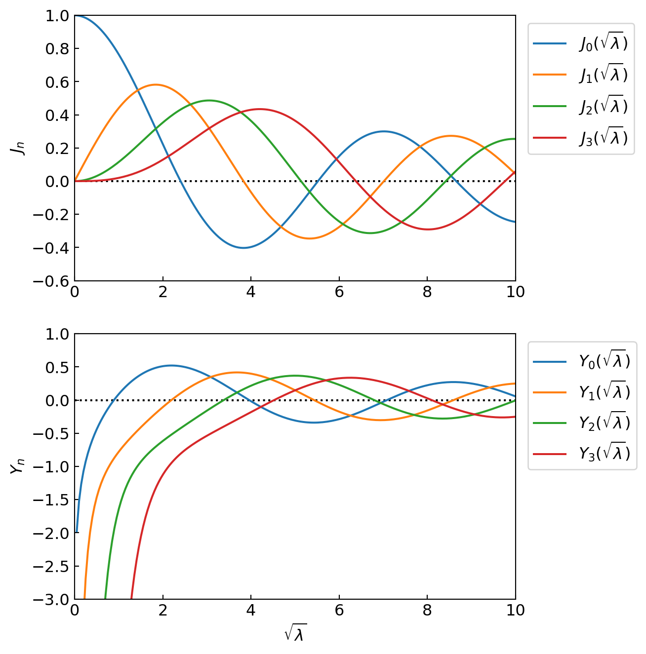
\(~\)
Since the functions \(Y_n(\sqrt{\lambda} r)\) are unbounded at \(r=0\), \(\,\)we choose as our solution \(J_n(\sqrt{\lambda} r)\). \(\,\)The last step in finding \(R_n(r)\) is to use the boundary condition \(R_n(1)=0~\) to find \(\lambda\). \(\,\)We must pick \(\lambda\) to be one of the roots of \(\,\color{red}{J_n(\sqrt{\lambda})=0}\); \(\,\)that is
\[\color{red}{\sqrt{\lambda_{nm}}=\alpha_{nm}}\]
where \(\,\alpha_{nm}\) is the \(m\)-th root of \(\,J_n(r)=0\), \(~m=1,2,3,\cdots\). \(\,\)With these roots, \(\,\)we have just solved the Helmholtz eigenvalue problem
The eigenvalues \(\,\lambda_{nm}\) are \(\,\alpha_{nm}^2\); \(\,\)and the corresponding eigenfunctions are
\[\color{red}{U_{nm}(r,\theta) =c_n J_n(\alpha_{nm} r) \cos (n\theta -\phi), \;\;\;n=0,1,2,\cdots, \;\;m=1,2,3,\cdots}\]
The general shape of \(\,U_{nm}(r,\theta)\,\) is the same for different values of the constants \(\,c_n\,\) and \(\,\phi.\) \(\,\)We plot these functions for the different values of \(\,n\) and \(\,m\) with \(\,c_n=1\,\) and \(\,\phi=0\)
\(~\)
ncols = 4
nrows = 4

fig, axs = plt.subplots(ncols=ncols,
    nrows=ncols, figsize=(7, 7),
    subplot_kw=dict(projection='polar'))

for ax in axs.flat:
    ax.set(xticks=[], yticks=[])

azimuths = np.radians(np.linspace(0, 360, 100))
zeniths = np.linspace(0, 1, 100)

theta, r = np.meshgrid(azimuths, zeniths)

for n in range(ncols):
    alpha_nm = jn_zeros(n, nrows)
    for m in range(nrows):
        U_nm = jv(n, alpha_nm[m] *r) *np.cos(n *theta)
        axs[n, m].contourf(theta, r, U_nm, levels=[0, 10])
        if m == 0:
            axs[n, 0].set_ylabel(f'n = {n}')
        if n == 0:
            axs[nrows -1, m].set_xlabel(f'm = {m +1}')

plt.show()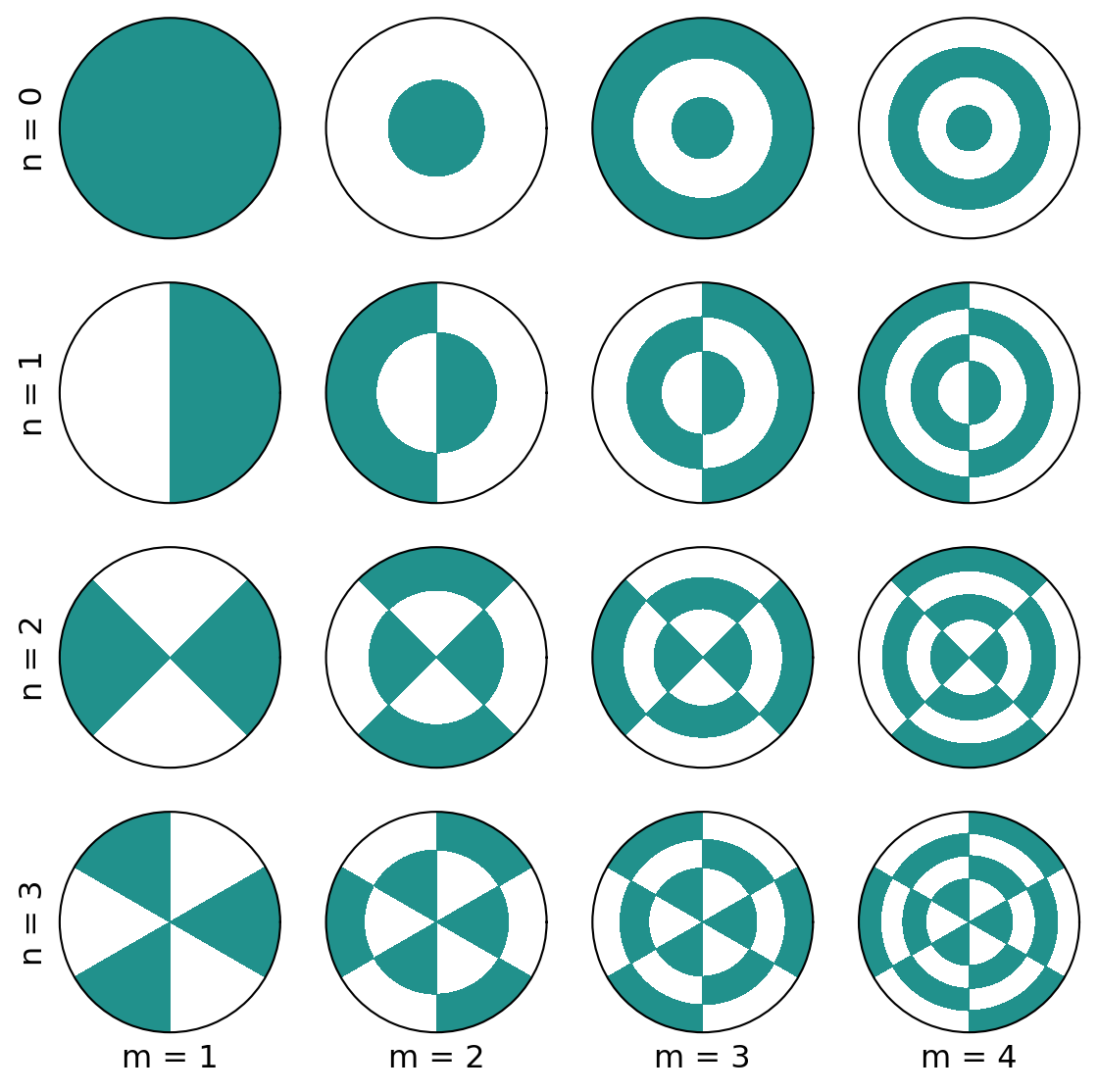
\(~\)
Now that we have solved the Helmholtz equation for the basic shapes \(\,U_{nm}(r,\theta)\), \(\,\)the final step is to multiply by the time factor
\[\color{red}{T_{nm}(t)=A_{nm}\cos c\alpha_{nm}t +B_{nm}\sin c\alpha_{nm} t}\]
and add the products in such a way that the initial conditions are satisfied. \(\,\)That is, \(\,\)the solution to our problem will be
\[ \color{red}{u(r,\theta,t) = \sum_{n=0}^\infty \sum_{m=1}^\infty J_n(\alpha_{nm}r) \cos n\theta \left[ A_{nm}\cos c\alpha_{nm}t +B_{nm}\sin c\alpha_{nm}t \right]}\]
Rather than going through the complicated process of finding \(\,A_{nm}\,\) and \(\,B_{nm}\,\) for the general case, \(\,\)we will find the solution for the situation where \(\,u\,\) is independent of \(\,\theta\) (very common, \(\,n=0\)). \(\,\)In other words, \(\,\)we will assume that the initial position of the drumhead depends only on \(\,r\)
In particular, \(\,\)we consider
\[\begin{aligned} u(r,\theta,0) &= \color{red}{f(r)}\\ u_t(r,\theta,0) &= 0 \end{aligned}\]
(It’s just easy to do the case where \(\,u_t \neq 0\)). \(\,\)With these assumptions, \(\,\)the solution now becomes
\[ u(r,t) = \sum_{m=1}^\infty A_{\color{red}{0}m} J_{\color{red}{0}}(\alpha_{\color{red}{0}m}r) \cos c\alpha_{\color{red}{0}m}t\]
and our goal is to find \(\,A_{0m}\,\) so that
\[ \color{blue}{f(r) = \sum_{m=1}^\infty \color{red}{A_{0m}} J_0(\alpha_{0m}r)} \tag{IC}\label{eq:IC}\]
To find the constants \(\,A_{0m}\), \(\,\)we use the orthogonality condition of the Bessel functions:
\[\int_0^1 rJ_0(\alpha_{0i} r)\,J_0(\alpha_{0j} r) \,dr = \begin{cases} 0 & i \neq j \\ \frac{1}{2}J_1^2(\alpha_{0i}) & i=j \end{cases}\]
Hence, \(\,\)we multiply each side of equation \(\eqref{eq:IC}\) by \(\,rJ_0(\alpha_{0j}r)\,\) and integrate from \(\,0\,\) to \(\,1\,\), \(\,\)giving
\[ \int_0^1 rf(r)J_0(\alpha_{0j}r)\,dr = A_{0j} \int_0^1 r J_0^2(\alpha_{0j}r)\,dr \]
from which we can solve for \(\,A_{0j}\)
\[ \color{red}{A_{0j}=\frac{2}{J_1^2(\alpha_{0j})} \int_0^1 rf(r)J_0(\alpha_{0j}r)\,dr, \;\;j =1,2,3,\cdots} \]
For example \(\,\)the solution to the vibrating drumhead with initial conditions
\[\begin{aligned} u(r,\theta,0) &= J_0(2.405 r) +0.5 J_0(8.654 r)\\ u_t(r,\theta,0) &= 0 \end{aligned}\]
would be
\[ u(r,t) = J_0(2.405 r) \cos(2.405 ct) +0.5 J_0(8.654 r)\cos(8.654 ct) \]
We start by drawing \(\,J_0(\sqrt{\lambda})\). \(\,\)Now, \(\,\)in order to graph the functions
\[J_0(\alpha_{01}r), \,J_0(\alpha_{02}r), \,\cdots,\, J_0(\alpha_{0m}r)\]
we rescale the \(\,r\)-axis so that \(\,m\)-th root passes through \(\,r=1\)
\(~\)
from mpl_toolkits.axisartist.axislines import SubplotZero

fig = plt.figure(figsize=(7, 8))
ax1 = SubplotZero(fig, 211)
ax2 = SubplotZero(fig, 212)

fig.add_subplot(ax1)
ax1.axis["left", "right", "bottom", "top"].set_visible(False)
ax1.axis["xzero", "yzero"].set_visible(True)
ax1.axis["xzero", "yzero"].set_axisline_style("-|>")

ax1.set_xticks([2, 4, 6, 8, 10])
ax1.set_ylim(-0.5, 1.1)
ax1.set_yticks([-0.5, 0.5, 1.0])
ax1.text(11, -0.03, r'$\sqrt{\lambda}$', fontsize=14)

fig.add_subplot(ax2)
ax2.axis["left", "right", "bottom", "top"].set_visible(False)
ax2.axis["xzero", "yzero"].set_visible(True)
ax2.axis["xzero", "yzero"].set_axisline_style("-|>")

ax2.set_xticks([0.2, 0.4, 0.6, 0.8, 1.0])
ax2.set_ylim(-0.5, 1.1)
ax2.set_yticks([-0.5, 0.5, 1.0])
ax2.text(1.1, -0.03, '$r$', fontsize=12)

mm = 3
alpha_0m =jn_zeros(0, mm)

r1 = np.linspace(0, 10, 100)
y1 = jv(0, r1)
ax1.plot(r1, y1, label=r'$J_0(\sqrt{\lambda})$')
ax1.plot(alpha_0m, np.zeros(mm), 'ro')

for m in range(mm):
    ax1.text(alpha_0m[m] -0.2, 0.1, rf'$\alpha_{{0{m +1}}}$', fontsize=12)
ax1.legend()

r2 = np.linspace(0, 1, 100)
for m in range(mm):
    y2 = jv(0, alpha_0m[m]*r2)
    ax2.plot(r2, y2, label=rf'$J_0(\alpha_{{0{m +1}}}r)$')
    ax2.plot(alpha_0m[:m +1] /alpha_0m[m], np.zeros(m +1), 'x')
ax2.legend()

plt.show() 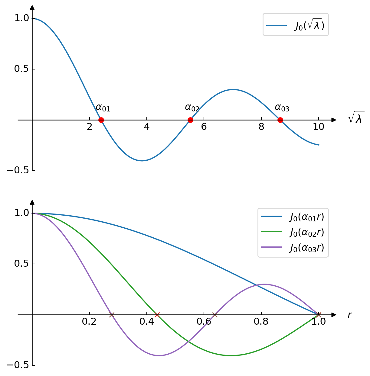
\(~\)
- In general, \(\,\)what we would do is to expand the initial position \(\,f(r)\,\) into the sum of these basic shapes \(\,J_0(\alpha_{0m} r)\), \(\,\)observe the vibration for each one and then add them up
fig = plt.figure(figsize=(7, 5))
ax = plt.axes(xlim=(0, 1), ylim=(-1.5, 1.5))

ax.set_xticks([0.0, 0.2, 0.4, 0.6, 0.8, 1.0])
ax.set_yticks([-1.5, -1.0, -0.5, 0, 0.5, 1.0, 1.5])
ax.tick_params(pad=10)
ax.set_xlabel('$r$')
ax.set_ylabel('$u(r,t)$')

plt.close()
line1, = ax.plot([], [], lw=1, ls=':')
line2, = ax.plot([], [], lw=1, ls=':')
line_sum, = ax.plot([], [], lw=4)
time_text = ax.text(0.45, 1.3, '')
def init():
time_text.set_text('t = 0.0')
line1.set_data([], [])
line2.set_data([], [])
line_sum.set_data([], [])
return (line1, line2, line_sum)
c = 1
alpha_0m =jn_zeros(0, 3)
def animate(t):
time_text.set_text(f't = {t:.2f}')
r = np.linspace(0, 1, 100)
u1 = jv(0, alpha_0m[0] *r) *np.cos(c *alpha_0m[0] *t)
u2 = 0.5 *jv(0, alpha_0m[2] *r) *np.cos(c *alpha_0m[2] *t)
u_sum = u1 +u2
line1.set_data(r, u1)
line2.set_data(r, u2)
line_sum.set_data(r, u_sum)
return (line1, line2, line_sum)
tt = np.linspace(0, 10, 100)
anim = animation.FuncAnimation(fig, animate,
init_func=init, frames=tt, interval=200, blit=True)
HTML('<center>' + anim.to_html5_video() + '</center>')\(~\)
Example \(\,\)Solve the vibrating drum head problem
\[ \begin{aligned} u_{tt} &=\nabla^2 u && 0 < r < 1, \;\; 0 < t < \infty \\ \\ u(1,\theta,t) &=0 && 0 < t < \infty \\ \\ \begin{array}{r} u(r,\theta,0) \\ u_t(r,\theta,0) \end{array} & \begin{array}{l} = 1 -r^2 \\ =0 \phantom{-r^2} \end{array} && 0 \leq r \leq 1 \end{aligned}\]
\(~\)
13.9 Dimensionless Problems
The basic idea behind dimensionless analysis is that by introducing new (dimensionless) variables in a problem, \(\,\)the problem becomes purely mathematical and contains none of the physical constants that originally characterized it
In this way, \(\,\)many different equations in physics, biology, engineering, \(\,\)and chemistry that contain special nuances via physical parameters are all transformed into the same simple form
Converting a Diffusion Problem to Dimensionless Form
Suppose we start with the initial-boundary-value problem:
\[ \begin{aligned} u_t &=\alpha u_{xx} && 0 < x < L, \;\; 0 < t < \infty \\[5pt] \begin{array}{r} u(0,t) \\ u(L,t) \end{array} & \begin{array}{l} = T_1 \\ = T_2 \end{array} && 0 < t < \infty \\[5pt] u(x,0) &= \sin \frac{\pi x}{L} && 0 \leq x \leq L \end{aligned}\]
Our goal is to change this problem to a new equivalent formulation that has the properties
- No physical parameters (like \(\alpha\)) in the new equation
- The initial and boundary conditions are simpler
\(~\)
Transforming the Dependent Variable \(~u \to U =\displaystyle\frac{u(x,t) -T_1}{T_2 -T_1}\)
\[ \begin{aligned} U_t &=\alpha U_{xx} && 0 < x < L, \;\; 0 < t < \infty \\[5pt] \begin{array}{r} U(0,t) \\ U(L,t) \end{array} & \begin{array}{l} = 0 \\ = 1 \end{array} && 0 < t < \infty \\[5pt] U(x,0) &= \frac{\displaystyle \sin \frac{\pi x}{L} -T_1}{T_2 -T_1} && 0 \leq x \leq L \end{aligned}\]
\(~\)
Transforming the Space Variable \(~x \to \xi=\;^{\displaystyle x}/_{\displaystyle L}\)
\[ \begin{aligned} U_t &=\frac{\alpha}{L^2} U_{\xi\xi} && 0 < \xi < 1, \; 0 < t < \infty \\[5pt] \begin{array}{r} U(0,t) \\ U(1,t) \end{array} & \begin{array}{l} = 0 \\ = 1 \end{array} && 0 < t < \infty \\[5pt] U(\xi,0) &= \frac{\sin\pi\xi -T_1}{T_2 -T_1} && 0 \leq \xi \leq 1 \end{aligned}\]
\(~\)
Transforming the Time Variable \(\;\; t \to \tau\)
Since our goal is to eliminate the constant \(\displaystyle\frac{\alpha}{L^2}\) from the PDE, \(\,\)we proceed as follows:
Try a transformation of the form \(\tau=ct\), \(\,\)where \(c\) is an unknown constant
Compute \(U_t=U_\tau\tau_t=cU_\tau\)
Substitute this derivative into the the PDE to obtain
\[cU_\tau =\frac{\alpha}{L^2} U_{\xi\xi}\]
and, \(\,\)hence, \(\,\)pick \(\displaystyle c=\frac{\alpha}{L^2}\). This give us our new time
\[ \tau=\frac{\alpha}{L^2} t \]
We now have the completely dimensionless problem
\[ \begin{aligned} U_\tau &= U_{\xi\xi} && 0 < \xi < 1, \; 0 < \tau < \infty \\[5pt] \begin{array}{r} U(0,\tau) \\ U(1,\tau) \end{array} & \begin{array}{l} = 0 \\ = 1 \end{array} && 0 < t < \infty \\[5pt] U(\xi,0) &= \frac{\sin\pi\xi -T_1}{T_2 -T_1} && 0 \leq \xi \leq 1 \end{aligned}\]
\(~\)
Transforming a Hyperbolic Problem to Dimensionless Form
Consider the vibrating string
\[ \begin{aligned} u_{tt} &=c^2 u_{xx} && 0 < x < L,\;\; 0 < t < \infty \\[5pt] \begin{array}{r} u(0,t) \\ u(L,t) \end{array} & \begin{array}{l} = 0 \\ = 0 \end{array} && 0 < t < \infty \\[5pt] \begin{array}{r} u(x,0) \\ u_t(x,0) \end{array} & \begin{array}{l} = \sin \frac{\pi x}{L} +0.5\sin \frac{3\pi x}{L} \\ = 0 \end{array} && 0 < x < L \end{aligned}\]
By transforming the independent variables (no need to transform \(u\)) into a new ones
\[ \xi=\frac{x}{L}\; \text{ and } \;\tau=\frac{c}{L} t \]
we get the new problem
\[ \begin{aligned} u_{\tau\tau} & =u_{\xi\xi} && 0 < \xi < 1,\;\; 0 < \tau < \infty \\[5pt] \begin{array}{r} u(0,\tau) \\ u(1,\tau) \end{array} & \begin{array}{l} = 0 \\ = 0 \end{array} && 0 < \tau < \infty \\[5pt] \begin{array}{r} u(\xi,0) \\ u_\tau(\xi,0) \end{array} & \begin{array}{l} = \sin \pi\xi +0.5\sin 3\pi\xi \\ = 0 \end{array} && 0 < \xi < 1 \\ \end{aligned}\]
which has the solution
\[ u(\xi,\tau)=\cos \pi \tau \sin\pi\xi +0.5 \cos 3\pi \tau \sin 3\pi \xi \]
\(~\)
Example \(\,\)How could you pick a new space variable \(\,\xi\,\) so that \(\,v\) is eliminated in the equation
\[ u_t +vu_x=0 \]
\(~\)
13.10 \(~\)Classification of PDEs (Cannonical Form of the Hyperbolic Equation)
The purpose here is to classify the second-order linear PDE
\[ \color{red}{A}u_{xx} +\color{red}{B}u_{xy} +\color{red}{C} u_{yy} +Du_x +Eu_y +Fu = G \tag{SL}\label{eq:SL}\]
in which \(A, B, C, D, E, F,\) and \(\,G\) are, in general, functions of \(x\) and \(y\) in two independent variables and could be constants, as
Hyperbolic if \(\,B^2 -4AC > 0~\) at \(\,(x,y)\)
Parabolic \(~\,\) if \(\,B^2 -4AC = 0~\) at \(\,(x,y)\)
Elliptic \(~~~~~\,\) if \(\,B^2 -4AC < 0~\) at \(\,(x,y)\)
and depending on which is true, \(\,\)the equation can be transformed into a corresponding cannonical (simple) form by introducing new coordinates \(\,\xi=\xi(x,y)\) \(\,\)and \(\,\eta=\eta(x,y)\)
\[\begin{aligned} u_{\xi\eta} = \Phi(\xi,\eta,u,u_\xi,u_\eta) \; &\text{ or } \; u_{\xi\xi} -u_{\eta\eta} = \Psi(\xi,\eta,u,u_\xi,u_\eta) \\ u_{\eta\eta} &= \Phi(\xi,\eta,u,u_\xi,u_\eta)\\ u_{\xi\xi} +u_{\eta\eta} &= \Phi(\xi,\eta,u,u_\xi,u_\eta) \end{aligned}\]
The student should note that whether equation \(\eqref{eq:SL}\) is hyperbolic, parabolic, or elliptic depends only on the coefficients of the second derivatives. \(\,\)We now come to the major portion of this section; \(\,\)rewriting hyperbolic equations in their canonical form
The Canonical Form of the Hyperbolic Equation
The objective here is to introduce new coordinates \(\,\xi=\xi(x,y)\,\) and \(\,\eta=\eta(x,y)\,\) so that the general PDE contains only one second derivative \(\,u_{\xi\eta}\,\). \(\,\)First of all, \(\,\)we compute the partial derivatives
\[\begin{aligned} Au_{xx} +Bu_{xy} +C u_{yy} &+Du_x +Eu_y +Fu = G \\ &\Downarrow\;\; \color{red}{\xi=\xi(x,y), \;\eta=\eta(x,y)} \\ u_x =\; u_\xi &\xi_x +u_\eta \eta_x \\ u_y =\; u_\xi &\xi_y +u_\eta \eta_y \\ u_{xx} =\; u_{\xi\xi}& \xi_x^2 +2u_{\xi\eta}\xi_x\eta_x +u_{\eta\eta}\eta_x^2 +u_\xi\xi_{xx} +u_\eta\eta_{xx}\\ u_{xy} =\;u_{\xi\xi}& \xi_x\xi_y +u_{\xi\eta}(\xi_x\eta_y +\xi_y\eta_x) +u_{\eta\eta}\eta_x\eta_y +u_\xi\xi_{xy} +u_\eta\eta_{xy}\\ u_{yy} =\;u_{\xi\xi}& \xi_y^2 +2u_{\xi\eta}\xi_y\eta_y +u_{\eta\eta}\eta_y^2 +u_\xi\xi_{yy} +u_\eta\eta_{yy}\\[5pt] &\Downarrow \\ \end{aligned}\]
\[ \begin{aligned} {\color{red}{\bar{A}}}u_{\xi\xi} +{\color{red}{\bar{B}}}u_{\xi\eta} +&{\color{red}{\bar{C}} u_{\eta\eta}} +\bar{D}u_\xi +\bar{E}u_\eta +\bar{F}u = \bar{G} \\[5pt] \text{in which} & \\[5pt] \bar{A}=&\;A\xi_x^2 +B\xi_x \xi_y +C\xi_y^2 \\ \bar{B}=&\;2A\xi_x\eta_x +B(\xi_x \eta_y+\xi_y\eta_x) +2C\xi_y\eta_y \\ \bar{C}=&\;A\eta_x^2 +B\eta_x \eta_y +C\eta_y^2 \\ % \bar{D}=&\;A\xi_{xx} +B\xi_{xy} % +C\xi_{yy} +D\xi_x +E\xi_y \\ % \bar{E}=&\;A\eta_{xx} +B\eta_{xy} % +C\eta_{yy} +D\eta_x +E\eta_y \\ % \bar{F}=&\;F\\ % \bar{G}=&\;G\\ \Downarrow& \\ \begin{pmatrix} 2\bar{A}& \bar{B}\\ \bar{B}& 2\bar{C} \end{pmatrix} =& \; \begin{pmatrix} \xi_x & \xi_y\\ \eta_x & \eta_y \end{pmatrix} \begin{pmatrix} 2A & B\\ B & 2C \end{pmatrix} \begin{pmatrix} \xi_x & \xi_y\\ \eta_x & \eta_y \end{pmatrix}^T \\ \Downarrow& \\ \bar{B}^2 -4\bar{A}\bar{C} =& \; (\xi_x\eta_y-\xi_y\eta_x)^2(B^2 -4AC) \\ =& \; J^2(B^2 -4AC) \end{aligned}\]
in which \(\,J\,\) is the Jacobian of the transformation and we select the transformation \(\,(\xi,\eta)\,\) such that \(\,J \neq 0\)
The next step in our process is to set the coefficients \(\,\bar{A}\,\) and \(\,\bar{C}\,\) to zero and solve for the tranformation \(\,\xi\,\) and \(\,\eta\,\). \(\,\)This will give us the coordinates that reduce the original PDE to canonical form:
\[\begin{aligned} \bar{A}=&\;A\xi_x^2 +B\xi_x \xi_y +C\xi_y^2 =0\\ \bar{C}=&\;A\eta_x^2 +B\eta_x \eta_y +C\eta_y^2 =0\\ &\Downarrow \\ A\left[ \frac{\xi_x}{\xi_y} \right]^2 &+B\left[ \frac{\xi_x}{\xi_y} \right] +C=0,\;\; A\left[ \frac{\eta_x}{\eta_y} \right]^2 +B\left[ \frac{\eta_x}{\eta_y} \right] +C=0 \\ &\Downarrow \\ \left[ \frac{\xi_x}{\xi_y} \right] =&\frac{-B +\sqrt{\color{blue}{B^2-4AC}}}{2A},\;\; \left[ \frac{\eta_x}{\eta_y} \right] =\frac{-B -\sqrt{\color{blue}{B^2-4AC}}}{2A} \end{aligned}\]
We have now reduced the problem to finding the two functions \(\,\xi(x,y)\,\) and \(\,\eta(x,y)\,\) so that their ratio \(\,[\xi_x/\xi_y]\,\) and \(\,[\eta_x/\eta_y]\,\) satisfy the above equation. \(\,\)Finding functions satisfying these conditions is really quite easy once we look for a few moments at figure

\[\begin{aligned} &\big\Downarrow \;\;{\scriptsize \xi = \text{constant}, \eta = \text{constant}}\\ \frac{dy}{dx} &=-\left[ \frac{\xi_x}{\xi_y} \right]=\frac{B -\sqrt{B^2-4AC}}{2A} =g_1(x,y)\\ \frac{dy}{dx} &=-\left[ \frac{\eta_x}{\eta_y} \right]=\frac{B +\sqrt{B^2-4AC}}{2A} =g_2(x,y)\\ &\Downarrow \;\;{\scriptsize \text{integration and arrangement}}\\ G_1(&x,y) = c_1 \\ G_2(&x,y) = c_2 \\ &\Downarrow \\ \xi &=G_1(x,y) \\ \eta &=G_2(x,y) \end{aligned}\]
\(~\)
Example \(\,\)Consider the simple equation
\[u_{xx} -4u_{yy} +u_x =0,\;\;\;B^2 -4AC=16>0\]
whose characteristic equations are
\[\begin{aligned} \frac{dy}{dx} &=-\left[ \frac{\xi_x}{\xi_y} \right]=\frac{B -\sqrt{B^2-4AC}}{2A} =-2\\ \frac{dy}{dx} &=-\left[ \frac{\eta_x}{\eta_y} \right]=\frac{B +\sqrt{B^2-4AC}}{2A} =2\\ \end{aligned}\]
To find \(\xi\) and \(\eta\), \(\,\)we first integrate for \(x\) and solve for the constants \(c_1\) and \(c_2,\) \(\,\) getting
\[\begin{array}{l} y =-2x+c_1 \\ y = 2x+c_2 \\ \end{array} \;\;\Rightarrow\;\; \begin{array}{l} \xi =y+2x=c_1 \\ \eta =y-2x=c_2 \end{array}\]

\(~\)
Example \(\,\)Suppose we start with the equation
\[y^2u_{xx} -x^2 u_{yy}=0,\;\;\;x>0,\;y>0\]
which is a hyperbolic equation in the first quadrant. \(\,\)We consider the problem of finding new coordinates that will change the original equation to canonical form for \(\,x\,\) and \(\,y\,\) in the first quadrant
STEP 1 \(\,\) Solve the two characteristic equations
\[\begin{aligned} \frac{dy}{dx} &=-\left[ \frac{\xi_x}{\xi_y} \right]=\frac{B -\sqrt{B^2-4AC}}{2A} =-\frac{x}{y}\\ \frac{dy}{dx} &=-\left[ \frac{\eta_x}{\eta_y} \right]=\frac{B +\sqrt{B^2-4AC}}{2A} =\frac{x}{y}\\ \end{aligned}\]
Integrating these two equations by the ODE technique of separating variables gives the implicit relationship
\[\begin{aligned} y^2 &-x^2 = c_1 \\ y^2 &+x^2 = c_2 \\ &\Downarrow \\ \xi= \,&y^2 -x^2 \\ \eta = \,&y^2 +x^2 \end{aligned}\]

We substitute this new coordinate into the equation to find the new equation
\[\begin{aligned} y^2 u_{xx} &-x^2 u_{yy}= 0\\ &\Downarrow\;\; \xi=y^2 -x^2,\; \eta=y^2 +x^2 \\ -16x^2y^2 u_{\xi\eta} -2(x^2 +y^2) &u_\xi +2(y^2 -x^2) u_\eta=0 \end{aligned}\]
STEP 2 \(\,\) Finally, \(\,\)solving for \(\,x\,\) and \(\,y\,\) in terms of \(\,\xi\,\) and \(\,\eta\), \(\,\)we get
\[ u_{\xi\eta}=\frac{\eta u_\xi -\xi u_\eta}{2(\xi^2 -\eta^2)}\]
\(~\)
Example \(\,\)Find the new characteristic coordinates for
\[u_{xx} + 4u_{xy} = 0\]
Solve the transformed equation in the new coordinate system and then transform back to the original coordinates to find the solution to the original problem
\(~\)
NOTES
The general hyperbolic equation actually has two canonical forms; \(\,\)the other one can be found by making yet another transformation
\[\begin{aligned} \alpha &=\xi +\eta \\ \beta &=\xi -\eta \end{aligned}\]
and rewriting the first canonical form in terms of \(\,\alpha\,\) and \(\,\beta\). \(\,\)The partial derivatives are transformed as follows:
\[\begin{aligned} u_\xi&= u_\alpha \alpha_\xi +u_\beta \beta_\xi=u_\alpha +u_\beta\\ u_\eta&= u_\alpha \alpha_\eta +u_\beta \beta_\eta=u_\alpha -u_\beta\\ u_{\xi\eta}&= u_{\alpha\alpha}\alpha_\eta +u_{\alpha\beta}\beta_\eta +u_{\beta\alpha}\alpha_\eta +u_{\beta\beta} \beta_\eta =u_{\alpha\alpha} -u_{\beta\beta} \end{aligned}\]
In the general parabolic equation, \(\,\)we obtain only a single canonical transformation as
\[ \bar{A}=0, \;\;\frac{dy}{dx}=-\left [ \frac{\xi_x}{\xi_y} \right ],\;\;\;\text{or}\;\;\; \bar{C}=0, \;\;\frac{dy}{dx}=-\left [ \frac{\eta_x}{\eta_y} \right ]\]
Suppose \(\,\xi\,\) is calculated. \(\,\)What could be the possible choice for \(\,\eta\,\)? \(\,\)We can select \(\,\eta\,\) as any arbitrary function of \(\,x\,\) and \(\,y\,\) such that \(\,\eta\,\) is independent of \(\,\xi\,\) (\(J \neq 0\))
In the general elliptic case, \(\,A\lambda^2 +B\lambda +C=0\,\) leads to complex conjugate canonical tramsformation \(\,\xi\,\) and \(\,\eta\). \(\,\)Since \(\,\xi\,\) and \(\,\eta\,\) are complex, \(\,\)we introduce new real variables
\[\begin{aligned} \alpha &= \frac{1}{2}(\xi +\eta)\\ \beta &= \frac{1}{2i}(\xi -i\eta) \end{aligned}\]
Under the transformation \(\,(x, y)\to (\alpha, \beta)\), \(\,\)the canonical form is given by
\[ u_{\alpha\alpha} +u_{\beta\beta}=\Phi(\alpha,\beta,u,u_\alpha,u_\beta)\]
The three major classifications of linear PDEs as hyperbolic, parabolic, and elliptic equations essentially classify physical problems into three basic physical types:
- Wave propagation
- Diffusion
- Steady-state problems
The mathematical solutions of these three types of equations are quite different
\(~\)
13.11 \(~\)First-Order Equations (Method of Characteristics)
If the student recalls, \(\,\)when we solved the diffusion equation
\[ u_t=\alpha u_{xx} - vu_x, \quad -\infty < x < \infty, \;\; 0 < t < \infty\]
the constant \(\,\alpha\,\) stood for the amount of diffusion, \(\,\)while \(v\) stood for the velocity of the medium
Hence if \(\,\alpha=0\) (no diffusion), \(\,\)it is clear (since we only have convection) that the solution will travel along the \(\,x\)-axis with velocity \(\,v\). \(\,\)In other words, \(\,\)if the initial solution is \(\,u(x,0)=\phi(x)\), \(\,\)then the solution to
\[u_t=-vu_x\]
would be \(\,u(x,t)=\phi(x-vt)\)
So we can think of the first-order equation
\[a(x,t)u_x +b(x,t)u_t = 0\]
as the concentration along a stream where the velocity is given by
\[ v=\frac{a(x,t)}{b(x,t)}\]
The purpose of this section is to introduce the notion of first-order partial differential equations and method of characteristics. \(\,\)The problem we will solve is the initial-value problem
\[ a(x,t) u_x +b(x,t) u_t +c(x,t)u=0 \]
\[u(x,0)=\phi(x), \;\; {-\infty<x<\infty,\;\; 0< t < \infty}\]
The solution to this equation is based on a physical fact, \(\,\)that an initial disturbance at some point \(\,x\,\) propagates along a line (curve) in the \(\,tx\)-plane (called a characteristic)

With this in mind, \(\,\)the idea is to introduce two new coordinates \(\,s\,\) and \(\,\tau\) (to replace \(\,x\,\) and \(\,t\)) that have the properties
- \(s\,\) will change along the characteristic curves
- \(\tau\,\) will change along the initial curve (most likely the line \(\,t=0\))
\[\begin{aligned} a(x,t) u_x +\, & b(x,t) u_t +c(x,t)u = 0\\ &\big\Downarrow\;\; {\scriptsize\text{characteristic curves } \{ \left( x(s), t(s) \right) : 0<s<\infty \}} \\ \frac{dx}{ds} = a(x,t), &\; \frac{dt}{ds} = b(x,t) \\ &\Downarrow \\ \frac{du}{ds}= u_x \frac{dx}{ds} +u_t\frac{dt}{ds}&=a(x,t) u_x +b(x,t) u_t \\ &\Downarrow \\ \frac{du}{ds} +\, &c(x,t)u =0 \end{aligned}\]
\(~\)
Example \(\,\)Solve the following IVP with constant coefficients:
\[ \begin{aligned} u_x +u_t +2u &=0 && -\infty < x < \infty,\;\; 0 < t < \infty \\ u(x,0) &=\sin x && -\infty < x < \infty \end{aligned}\]
STEP 1 \(\,\) Find the characteristics (along which the initial data propagate)
\[\begin{aligned} \frac{dx}{ds}=1,\;\; \frac{dt} {ds}&=1\quad 0<s<\infty \\ &\Downarrow \\ x(s) = &\;s +c_1 \\ t(s) = &\;s +c_2 \\ &\Downarrow \;\;x(0)= \tau, \;\;t(0)=0 \\ x = &\;s +\tau \\ t = &\;s \\ &\Downarrow \\ x - t = \tau, \;\;\;&-\infty < \tau < \infty \end{aligned}\]

STEP 2 \(\,\) Using this coordinate system, \(\,\)we change the PDE to the ODE
\[\begin{aligned} \frac{du}{ds} +2u&= 0, \;\; u(0)= \sin\tau \\ &\Downarrow \\ u(s,\tau) &=\sin \tau \cdot e^{-2s} \end{aligned}\]
STEP 3 \(\,\) We now solve the transformation for \(\,s\,\) and \(\,\tau\,\) in terms of \(\,x\,\) and \(\,t\):
\[u(x,t) = \sin(x -t) \cdot e^{-2t}\]

\(~\)
Example \(\,\)Solve the following IVP with variable coefficients:
\[ \begin{aligned} x u_x +u_t +tu &=0 && -\infty < x < \infty,\; 0 < t < \infty \\ u(x,0) &=F(x) && -\infty < x < \infty, \;\;\text{an arbitrary initial wave} \end{aligned}\]
STEP 1 \(\,\) Find the characteristics (along which the initial data propagate)
\[\begin{aligned} \frac{dx}{ds} =x,\;\;&\frac{dt}{ds} =1 \quad 0<s<\infty \\ &\Downarrow \\ x(s) &=\; c_1 e^s\\ t(s) &=\; s +c_2 \\ &\Downarrow \;\; x(0)= \tau, \;\;t(0)=0 \\ x &=\;\tau e^s \\ t &=\;s \end{aligned}\]
STEP 2 \(\,\) Using this coordinate system, \(\,\)we change the PDE to the ODE
\[\begin{aligned} \frac{du}{ds} +su&= 0, \;\; u(0)= F(\tau) \\ &\Downarrow \\ u(s,\tau) &=F(\tau) \cdot e^{-s^2/2} \end{aligned}\]
STEP 3 \(\,\) We now solve the transformation for \(\,s\,\) and \(\,\tau\,\) in terms of \(\,x\,\) and \(\,t\)
\[u(x,t) = F(xe^{-t}) \cdot e^{-t^2/2}\]
\(~\)
Example \(\,\) Solve the problem in higher dimensions (surface waves)
\[ \begin{aligned} a u_x +b u_y +c u_t +du &=0 && \scriptsize -\infty < x < \infty, \;-\infty < y < \infty, \; 0< t < \infty \\ u(x,y,0) &=e^{-(x^2 +y^2)} && \scriptsize -\infty < x < \infty, \;-\infty < y < \infty \end{aligned}\]
\(~\)
13.12 \(~\)Nonlinear First-Order Equations (Conservation Equations)
One of the most useful partial differential equations in mathematics is the conservation equation
\[u_t +f_x=0\]
This equation says that the increase of a physical quantity \(\,u_t\,\) is equal to the change in flux \(\,-f_x\,\) of that quantity across the boundary
Derivation of the Conservation Equation
Suppose we have a stretch of highway on which cars are moving from left to right, \(\,\)and we assume there are no exit and entrance ramps. \(\,\)We let
\[ \begin{aligned} u(x,t) &=\text{density of cars at } x\;\; (\text{cars per unit length at } x) \\[5pt] f(x,t) &=\text{flux of cars at } x \;\; (\text{cars per minute passing the point } x) \end{aligned}\]
Then, \(\,\)it is fairly obvious that for a road segment \(\,[a,b]\), \(\,\)the change in the number of cars (with respect to time) is given by both of the following expressions:
\[\begin{aligned} \text{change in the number of cars in } [a,b] &= \frac{d}{dt} \int_a^b u(x,t)\,dx \\ \text{change in the number of cars in } [a,b] &= f(a,t) -f(b,t) = -\int_a^b \frac{\partial f}{\partial x}(x,t)\,dx \end{aligned}\]
Setting these two integrals equal to each other, \(\,\)we have
\[ \int_a^b \frac{\partial u}{\partial t}(x,t)\,dx = -\int_a^b \frac{\partial f}{\partial x}(x,t)\,dx\]
Finally, \(\,\)since the integral \(\,[a,b]\,\) was arbitrary, \(\,\)we have the one-dimensional conservation equation
\[u_t +f_x=0\]
If we carried out a similar analysis in two or three dimensions, \(\,\)we would have
\[u_t +f_x +f_y=0, \;\; u_t +f_x +f_y +f_z=0\]
\(~\)
Conservation Equation Applied to the Traffic Problem
We are now ready to see how the conservation equation \(\,u_t +f_x=0\,\) can be applied to the traffic problem
To do this, \(\,\)we rewrite the change in flux \(\,f_x\,\) as
\[f_x = \frac{df}{du} u_x,\;\;\text{chain rule}\]
and substitute it in the conservation equation. \(\,\)Doing this, \(\,\)we arrive at
\[ u_t +\frac{df}{du}u_x=u_t+g(u)u_x=0\]
where we can imagine a car moving upstream or downstream with velocity \(\,g(u)\)
Hence, after \(\,t\,\) minutes, the position \(\,x\,\) of the car will be
\[x = x_0 +g(u)t, \quad\text{characteristic equation}\]
Remembering that the concentration \(\,u(x,t)\,\) will not change along each characteristic, \(\,\)if we know the initial density \(\,u(x_0,0)\), then the characteristic equation for \(\,x\,\) can be written
\[x=x_0+g[u(x_0,0)]t\]
- It is clear that by knowing these characteristic curves starting from each point (and knowing the solution doesn’t change along these curves), \(\,\)we can piece together the solution \(\,u(x,t)\,\) for all time \(\,t\). \(\,\)We won’t actually find the explicit equation for the solution \(\,u(x,t)\,\) in terms of \(\,x\,\) and \(\,t\,\) but will use our knowledge of the characteristics of the equation to solve some interesting problems

\(~\)
Traffic-Flow Problem
- We will now solve a traffic-flow problem where the flux is given by \(\,f(u)=u^2\) and the initial density of cars is given. \(\,\)In other words, \(\,\)we have
\[ u_t +2uu_x =0 \quad -\infty < x < \infty, \; 0< t < \infty\]
\[u(x,0) = \begin{cases} \;\;\; 1 & x \leq 0\\ 1 -x & 0 < x < 1, \;-\infty < x <\infty \\ \;\;\; 0 & 1 \leq x \end{cases}\]

STEP 1
We begin by finding the characteristics starting from each initial point \(\,(x_0,0)\). \(\,\)For \(\,x_0 < 0\), \(\,\)the characteristics are
\[\begin{aligned} x &= x_0 +g[u(x_0,0)] t \\ &= x_0 +g[1] t\\ &= x_0 +2t \\ &\Downarrow \\ t &=\frac{1}{2} (x -x_0) \end{aligned}\]
Now consider those initial points \(\,0 < x_0 < 1\). \(\,\)Here, \(\,\)the characteristic curves are
\[\begin{aligned} x &= x_0 +g[u(x_0,0)] t \\ &= x_0 +g[1 -x_0] t\\ &= x_0 +2(1 -x_0)t \\ &\Downarrow \\ t &=\frac{x -x_0}{2(1 -x_0)} \end{aligned}\]
Finally, \(\,\)for \(\,1 \leq x_0 < \infty\), \(\,\)we have the characteristics
\[\begin{aligned} x &= x_0 +g[u(x_0,0)] t \\ &= x_0 +g[0] t\\ &= x_0 \end{aligned}\]
which represents vertical lines starting at \(\,x_0\)

The solution remains constant along each characteristic line. \(\,\)Now the solution for \(\,x \in \mathbb{R}\), \(\,0 \leq t <\textstyle\frac{1}{2}\,\) is given by
\[u(x,t)= \begin{cases} \quad 1 & \; x \leq 2t,\qquad 0 \leq t < \frac{1}{2}\\ \displaystyle\frac{1 -x}{1 -2t} & 2t \leq x < 1, \;\, 0 \leq t < \frac{1}{2} \\ \quad 0 & \; 1 \leq x, \qquad \; 0 \leq t < \frac{1}{2} \end{cases}\]
The difficulty in this example is that some characteristic lines will intersect each other. \(\,\)In other words, \(\,\)at the intersection point \(\,(1,\textstyle \frac{1}{2})\,\) of the two characteristic lines, \(\,\)the solution becomes multi-valued. \(\,\)This pathology means that the solution in the usual sense fails to exist after \(\,t \geq \textstyle \frac{1}{2}\)

STEP 2
Hence, \(\,\)to find the solution past \(\,t=\textstyle \frac{1}{2}\), \(\,\)we must use another type of analysis. \(\,\)When characteristics run together, \(\,\)we have the phenomenon of shock waves (discontinuous solutions), \(\,\)and what we must ask is, \(\,\)how fast does the leading edge of the shork wave propagate along the road?
Before proceeding further, \(\,\)it is necessary to introduce the concept of a jump condition: a condition that holds at a discontinuity or abrupt change. \(\,\)Consider one dimensional problem where there is a jump in the conserved quantity \(\,u\):
\[u_t +f_x=0\]
Let the solution exhibit a jump (or shork) at \(\,x=x_s(t)\,\) and integrate over the partial domain, \(\,x \in (x_1, x_2)\), \(\,\)where \(\,x_1 < x_s(t) < x_2\),
\[\scriptsize \begin{aligned} \frac{d}{dt} \left( \int_{x_1}^{x_s(t)}u\,dx +\int_{x_s(t)}^{x_2}u \,dx\right)&= -\int_{x_1}^{x_2} \frac{\partial } {\partial x} f(u)\,dx\\ &\Downarrow \\ \int_{x_1}^{x_s(t)} u_t \,dx +u^-(x_s(t),t)\frac{dx_s}{dt} +\int_{x_s(t)}^{x_2} u_t \,dx &-u^+(x_s(t),t)\frac{dx_s}{dt}= -\left. \underset{}{f(u)}\, \right|_{x_1}^{x_2}\\ x_1 \to x_s(t),\;x_2 \to x_s(t) \;\; &\Downarrow \\ \left[ u^-(x_s(t),t) -u^+(x_s(t),t) \right] \frac{d x_s}{dt} &= f(u^-(x_s(t),t)) -f(u^+(x_s(t),t)) \\ &\Downarrow \\ s=\frac{d x_s}{dt} &=\frac{f(u^-(x_s(t),t)) -f(u^+(x_s(t),t))}{ u^-(x_s(t),t) -u^+(x_s(t),t)} \end{aligned}\]
in which \(\,s\,\) is the speed of the discontinuity and represents the jump condition for conservation eqaution
A shork situation arises in a system where its characteristics intersect, \(\,\)and under these conditions a requirement for a unique single-valued solution is that the solution should satisfy the Lax entropy condition
\[f'(u^+(x_s(t),t)) < s < f'(u^-(x_s(t),t))\]
where \(f'(u^+(x_s(t),t))\,\) and \(\,f'(u^-(x_s(t),t))\,\) represent characteristic speeds at upstream and downstream conditions, respectively
So, \(\,\)in our example, \(\,\)the speed of the wave front would be(remembering that \(\,f(u)=u^2\))
\[ s = \frac{1 -0}{1 -0}=1\]
Therefore, \(\,\)a shock is formed at \((x,t)=(1,\textstyle\frac{1}{2})\):
After that, \(\,\)it moves with constant speed \(1\), \(\,\)along the line \(\,x=t +\textstyle \frac{1}{2}\), \(\,\)for \(\,t \geq \textstyle \frac{1}{2}\).
In conclusion, \(\,\)the solution takes different forms in the three different regions in the space-time plane
\[u(x,t)= \begin{cases} \quad 1 & x \leq 2t, \qquad\; 0 \leq t < \frac{1}{2} \;\;\text{or}\;\; x-\frac{1}{2} \leq t, \;\;t \geq \frac{1}{2}\\ \displaystyle\frac{1 -x}{1 -2t} & 2t \leq x < 1, \;\, 0 \leq t < \frac{1}{2} \\ \quad 0 & x \geq 1, \qquad\;\; 0 \leq t < \frac{1}{2} \;\;\text{or}\;\; x-\frac{1}{2} > t, \;\;t \geq \frac{1}{2} \end{cases}\]
\(~\)
Example \(\,\) Solve
\[ \begin{aligned} u_t +uu_x &=0 \qquad -\infty < x < \infty, \; 0 < t < \infty \\ u(x,0) &= \begin{cases} 3(1 -|x|) & |x| \leq 1\\ \quad\; 0 & |x| > 1 \end{cases} \end{aligned}\]
\(~\)
Example \(\,\) Verify that \(\,u=\phi[x-g(u)t]\,\) is an implicit solution of the nonlinear problem
\[ \begin{aligned} u_t +g(u)u_x &=0 \quad -\infty < x < \infty, \; 0 < t < \infty \\ u(x,0) &= \phi(x) \end{aligned}\]
\(~\)
13.13 \(~\)Systems of PDEs
In many areas of science, \(\,\)several unknown quantities (and their derivatives) are modeled by a system of interlocking equations. \(\,\)And we seek to find all of these functions simultaneously
There are other reasons for studying systems of equations. \(\,\)Although things are not quite so simple in PDE theory, \(\,\)it is often possible to write a single higher-order PDE as a system of first-order equations
For example, \(\,\)the telegraph equation
\[ u_{tt}=c^2u_{xx} +au_t +bu \]
can be rewritten in equivalent form as three first-order PDEs by introducing the three variables:
\[\begin{aligned} u_1 &= u \\ u_2 &= u_x \\ u_3 &= u_t \end{aligned}\]
It is a simple matter to see that the telegraph equation is equivalent to the three equations:
\[\begin{aligned} \frac{\partial u_1}{\partial x} &= u_2 \\[2pt] \frac{\partial u_1}{\partial t} &= u_3 \\[2pt] \frac{\partial u_3}{\partial t} &= c^2 \frac{\partial u_2}{\partial x} +au_3 +bu_1 \end{aligned}\]
Solution of the Linear System \(\,\mathbf{u}_t +\mathbf{A}\mathbf{u}_x=\mathbf{0}\)
Consider the initial-value problem consisting of two PDEs and two ICs
\[\begin{aligned} \frac{\partial u_1}{\partial t} +8 &\frac{\partial u_2}{\partial x} = 0 \\[2pt] \frac{\partial u_2}{\partial t} +2 &\frac{\partial u_1}{\partial x} = 0 \\[5pt] u_1(x,0)& = f(x) \\ u_2(x,0)& = g(x) \end{aligned}\]
We start by writing the two PDEs in matrix form
\[\begin{aligned} \begin{bmatrix} \frac{\partial u_1}{\partial t} \\ \frac{\partial u_2}{\partial t} \end{bmatrix} +&\begin{bmatrix} 0 & 8 \\ 2 & 0 \end{bmatrix} \begin{bmatrix} \frac{\partial u_1}{\partial x} \\ \frac{\partial u_2}{\partial x} \end{bmatrix} = \begin{bmatrix} 0 \\ 0 \end{bmatrix} \\ \end{aligned}\]
\[\begin{aligned} &\Downarrow \\[2pt] \mathbf{u}_t + &\mathbf{A}\mathbf{u}_x = \mathbf{0} \\[2pt] &\Downarrow \;\; \mathbf{u}=\mathbf{P}\mathbf{v}\\[2pt] \mathbf{v}_t +&\mathbf{P}^{-1} \mathbf{A}\mathbf{P}\mathbf{v}_x = \mathbf{0} \\[2pt] &\Downarrow \\[2pt] \mathbf{v}_t + &\boldsymbol{\Gamma}\mathbf{v}_x = \mathbf{0} \end{aligned}\]
where
\[\mathbf{P}= \begin{bmatrix} 2 & -2 \\ 1 & \;\;\,1 \end{bmatrix},\;\; \boldsymbol{\Gamma}= \begin{bmatrix} 4 & \;\;\,0 \\ 0 & -4 \end{bmatrix}\qquad\]
These are the two uncoupled equations that we can solve independently
\[\begin{aligned} &\frac{\partial v_1}{\partial t} +4\frac{\partial v_1}{\partial x} = 0 \\ &\frac{\partial v_2}{\partial t} -4\frac{\partial v_2}{\partial x} = 0 \end{aligned}\]
These equations have travelling-wave solutions
\[\begin{aligned} v_1(x,t) &= \phi(x -4t) \\ v_2(x,t) &= \psi(x +4t) \end{aligned}\]
where \(\,\phi\,\) and \(\,\psi\,\) are arbitrary differentiable functions
To obtain our general solution \(\,u\), \(\,\)we merely compute
\[\mathbf{u}=\mathbf{P}\mathbf{v}= \begin{bmatrix} 2\phi(x -4t) -2\psi(x+4t)\\ \phi(x -4t) +\psi(x+4t) \end{bmatrix}\]
We now substitute general solution into the ICs to get
\[\begin{aligned} 2\phi(x) &-2\psi(x) = f(x) \\ \phi(x) &+\psi(x) = g(x) \\ &\Downarrow \\ \phi(x) &= \frac{1}{4} \left[ f(x) +2g(x) \right] \\ \psi(x) &= \frac{1}{4} \left[ 2g(x) -f(x) \right] \end{aligned}\]
and, \(\,\)hence, \(\,\)the solution to IVP is
\[\begin{aligned} u_1(x,t) &= \frac{1}{2} \left[ f(x -4t) +2g(x -4t) \right] -\frac{1}{2}\left[ 2g(x +4t) -f(x +4t) \right]\\ u_2(x,t) &= \frac{1}{4} \left[ f(x -4t) +2g(x -4t) \right] +\frac{1}{4}\left[ 2g(x +4t) -f(x +4t) \right] \end{aligned}\]
\(~\)
Example \(\,\) What is the general solution of the system
\[\begin{aligned} &\frac{\partial u_1}{\partial t} +\frac{\partial u_1}{\partial x} +\frac{\partial u_2}{\partial x} = 0\\ &\frac{\partial u_2}{\partial t} +4\frac{\partial u_1}{\partial x} +\frac{\partial u_2}{\partial x} = 0 \end{aligned}\]
\(~\)
Worked Exercises
1. \(~\) Find \(u(0,0,0,t)\)
\[ \begin{aligned} u_{tt} &= \nabla^2 u, \;\; t > 0\\ &u(x, y, z, 0) = 0, \; u_t(x, y, z, 0) = x^2 +y^2 +z^2 \end{aligned} \]
Solution
Step 1: \(~\) Use the Kirchhoff’s formula (solution to 3D wave equation)
For the 3D wave equation (with wave speed \(c= 1\)), the solution with initial conditions \(u(\mathbf{x},0) = f(\mathbf{x})\), \(u_t(\mathbf{x},0) = g(\mathbf{x})\) is:
\[u(\mathbf{x},t) = \frac{1}{4\pi t} \int_{|\xi - \mathbf{x}| = t} g(\xi) \, dS(\xi) + \frac{1}{4\pi t^2} \int_{|\xi - \mathbf{x}| = t} f(\xi) \, dS(\xi) \]
where the integrals are over the sphere of radius \(t\) centered at \(\mathbf{x}\)
In our problem:
- \(f(x,y,z) = 0\)
- \(g(x,y,z) = x^2 + y^2 + z^2 = |\xi|^2\)
- Point of interest: \(\mathbf{x} = (0,0,0)\)
Thus:
\[u(0,0,0,t) = \frac{1}{4\pi t} \int_{|\xi| = t} |\xi|^2 \, dS(\xi)\]
Step 2: \(~\) Evaluate the integral
On the sphere \(|\xi| = t\), we have \(|\xi|^2 = t^2\) constant
Then:
\[u(0,0,0,t) = \frac{1}{4\pi t} \int_{|\xi| = t} t^2 \, dS(\xi) = \frac{t^2}{4\pi t} \cdot \text{Surface area of sphere of radius } t\]
The surface area of a sphere of radius \(t\) is \(4\pi t^2\), so:
\[u(0,0,0,t) = \frac{t^2}{4\pi t} \cdot 4\pi t^2 = t^2 \cdot t = \boxed{t^3}\]
\(~\)
2. \(~\) Find \(u(x,y,z,t)\)
\[ \begin{aligned} u_{tt} &= \nabla^2 u, \;\; t > 0\\ &u(x, y, z, 0) = 0, \; u_t(x, y, z, 0) = x \end{aligned} \]
Solution
Step 1: \(~\) Use Kirchhoff’s formula (3D wave equation)
For the 3D wave equation \(u_{tt} = \nabla^2 u\) with wave speed \(c = 1\), the general solution with initial data
\[u(\mathbf{x},0) = f(\mathbf{x}), \quad u_t(\mathbf{x},0) = g(\mathbf{x})\]
is given by:
\[u(\mathbf{x},t) = \frac{1}{4\pi t} \int_{|\xi - \mathbf{x}| = t} g(\xi) \, dS(\xi) + \frac{1}{4\pi t^2} \int_{|\xi - \mathbf{x}| = t} f(\xi) \, dS(\xi)\]
In our case:
- \(f(x,y,z) = 0\)
- \(g(x,y,z) = x\) (we’ll write this as \(\xi_1\) to distinguish from the field point \(\mathbf{x} = (x_1,x_2,x_3)\))
- Therefore:
\[u(\mathbf{x},t) = \frac{1}{4\pi t} \int_{|\xi - \mathbf{x}| = t} \xi_1 \, dS(\xi)\]
Step 2: \(~\) Use coordinate shift
Let’s simplify by performing a change of variables to center the sphere
Let \(\mathbf{x} = (x_1, x_2, x_3)\), and let \(\xi = \mathbf{x} + t\omega\), where \(\omega \in S^2\) is a unit vector. Then \(|\xi - \mathbf{x}| = t\), and \(dS(\xi) = t^2\, d\omega\). So:
\[u(\mathbf{x},t) = \frac{1}{4\pi t} \int_{|\xi - \mathbf{x}| = t} \xi_1 \, dS(\xi) = \frac{1}{4\pi t} \int_{S^2} (x_1 + t\omega_1) \cdot t^2 \, d\omega\]
Simplify:
\[u(\mathbf{x},t) = \frac{t}{4\pi} \int_{S^2} (x_1 + t\omega_1) \, d\omega = \frac{t}{4\pi} \left[ x_1 \int_{S^2} d\omega + t \int_{S^2} \omega_1 \, d\omega \right]\]
Now compute the integrals:
\(\displaystyle \int_{S^2} d\omega = 4\pi\)
\(\displaystyle \int_{S^2} \omega_1 \, d\omega = 0~\) (odd function over symmetric sphere)
So:
\[u(\mathbf{x},t) = \frac{t}{4\pi} \cdot x_1 \cdot 4\pi = x_1 t = x t\]
\(~\)
3. \(~\) Solve the vibrations of a membrane which is in the \(xy\) plane:
\[ \begin{aligned} u_{tt} &= \frac{\rho}{T} \left[ \frac{\partial^2 u}{\partial x^2} +\frac{\partial^2 u}{\partial y^2} \right] , \;\; 0 < x < \pi, \;0 < y < \pi \\ u&(0, y, t) =0, \; u(\pi, y, t) =0 \\ u&(x, 0, t) =0, \; u(x, \pi, t) =0 \\ u&(x,y,0) = \sin 2x \sin 3y +\sin 3x \sin2y. \; u_t(x,y,0) =0 \end{aligned}\]
Solution
Step 1: \(~\) Separation of Variables
Assume a solution of the form: \[u(x, y, t) = X(x) Y(y) T(t)\] Plugging into the wave equation:
\[X Y T'' = c^2 \left( X'' Y T + X Y'' T \right)\]
Divide both sides by \(XYT\):
\[\frac{T''}{c^2 T} = \frac{X''}{X} + \frac{Y''}{Y} = -\lambda\]
We separate variables: \[\frac{X''}{X} + \frac{Y''}{Y} = -\lambda \Rightarrow \begin{cases} X’’ + \mu X = 0 \\ Y’’ + (\lambda - \mu) Y = 0 \end{cases}\]
With the boundary conditions: \[\begin{aligned} X(0) &= X(\pi) = 0 \Rightarrow X_n(x) = \sin(nx),\quad \mu = n^2 \\ Y(0) &= Y(\pi) = 0 \Rightarrow Y_m(y) = \sin(my),\quad \lambda - \mu = m^2 \Rightarrow \lambda = n^2 + m^2 \end{aligned}\]
Then the time part: \[\begin{aligned} T'' &+ c^2(n^2 + m^2)T = 0\\ &\Rightarrow T_{n,m}(t) = A_{n,m} \cos(c\sqrt{n^2 + m^2}t) + B_{n,m} \sin(c\sqrt{n^2 + m^2}t) \end{aligned}\]
Step 2: \(~\) General Solution
\[ \begin{aligned} u(x, y, t) = \sum_{n=1}^{\infty} \sum_{m=1}^{\infty} &\left[ A_{n,m} \cos(c\sqrt{n^2 + m^2} t)\right. \\ &\left.+ B_{n,m} \sin(c\sqrt{n^2 + m^2} t) \right] \sin(nx) \sin(my) \end{aligned} \]
Step 3: \(~\) Apply Initial Conditions
Initial displacement:
\[u(x, y, 0) = \sum_{n,m} A_{n,m} \sin(nx)\sin(my) = \sin 2x \sin 3y + \sin 3x \sin 2y\]
So \(A_{2,3} = 1\), \(A_{3,2} = 1\), all others zero
Initial velocity: \[u_t(x, y, 0) = -c\sum_{n,m} c\sqrt{n^2 + m^2} B_{n,m} \sin(nx)\sin(my) = 0 \Rightarrow B_{n,m} = 0\]
Final Answer
\[u(x, y, t) = \cos\left(c \sqrt{13}\, t\right) \sin(2x) \sin(3y) +\cos\left(c \sqrt{13}\, t\right) \sin(3x) \sin(2y)\]
where \(c = \sqrt{\rho/T}\)
\(~\)
import numpy as np
import matplotlib.pyplot as plt

def plot_rectangle_membrane_normal_modes(n, m):

    fig, ax = plt.subplots(figsize=(3, 3))

    ax.set(xticks=[], yticks=[])

    x_ = np.linspace(0, np.pi, 100)
    y_ = np.linspace(0, np.pi, 100)

    X_, Y_ = np.meshgrid(x_, y_)
    U_ = np.sin(n*X_) *np.sin(m*Y_) +np.sin(m*X_) *np.sin(n*Y_)

    ax.contourf(X_, Y_, U_, levels=[0, 10])

    ax.set_title(f'$n={n}$, $m={m}$')

plt.show()plot_rectangle_membrane_normal_modes(2, 3)
\(~\)
4. \(~\) Solve the vibrations of a membrane which is in the \(xy\) plane:
\[\begin{aligned} u_{tt} &= \frac{\rho}{T} \left[ \frac{\partial^2 u}{\partial x^2} +\frac{\partial^2 u}{\partial y^2} \right] , \;\; 0 < x < \pi, \;0 < y < \pi \\ u&(0, y, t) =0, \; u(\pi, y, t) =0 \\ u&(x, 0, t) =0, \; u(x, \pi, t) =0 \\ u&(x,y,0) = \sin x \sin 4y +\sin 4x \sin y, \; u_t(x,y,0) =0 \end{aligned}\]
Solution
Step 1: \(~\) Use Separation of Variables
Assume a solution of the form:
\[ \begin{aligned} u(x,y,t) = \sum_{n=1}^\infty \sum_{m=1}^\infty &\left[ A_{nm} \cos(c\sqrt{n^2 + m^2} \, t)\right.\\ &+\left. B_{nm} \sin(c\sqrt{n^2 + m^2} \, t) \right] \sin(nx) \sin(my) \end{aligned}\]
From the initial displacement: \[u(x,y,0) = \sum_{n,m} A_{nm} \sin(nx)\sin(my) = \sin x \sin 4y + \sin 4x \sin y\]
So the only nonzero coefficients are: \[A_{1,4} = 1,\quad A_{4,1} = 1\]
From the initial velocity condition: \[u_t(x,y,0) = 0 \Rightarrow B_{nm} = 0\]
Step 2: \(~\) Final Solution
\[\begin{aligned} u(x, y, t) &= A_{1,4} \cos(c \sqrt{1^2 + 4^2} \, t) \sin x \sin 4y\\ &\quad+ A_{4,1} \cos(c \sqrt{4^2 + 1^2} \, t) \sin 4x \sin y \\ &= \cos(c\sqrt{17} \, t) \sin x \sin 4y + \cos(c\sqrt{17} \, t) \sin 4x \sin y \end{aligned}\]
Thus, the solution is:
\[ u(x, y, t) = \cos(c\sqrt{17} \, t) \left[ \sin x \sin 4y + \sin 4x \sin y \right] \]
where \(c = \sqrt{\frac{\rho}{T}}\)
\(~\)
plot_rectangle_membrane_normal_modes(1, 4)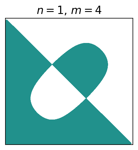
\(~\)
5. \(~\) Suppose the vibration of a string is described by \(u_{tt}=u_{xx}\) and has an initial displacement as given by the following diagram:
\((a)\)
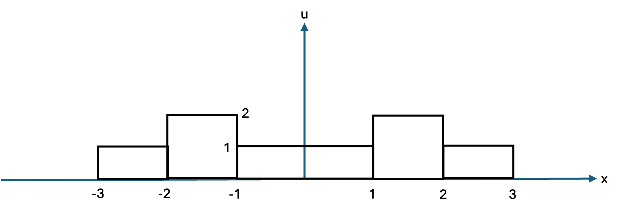
\((b)\)
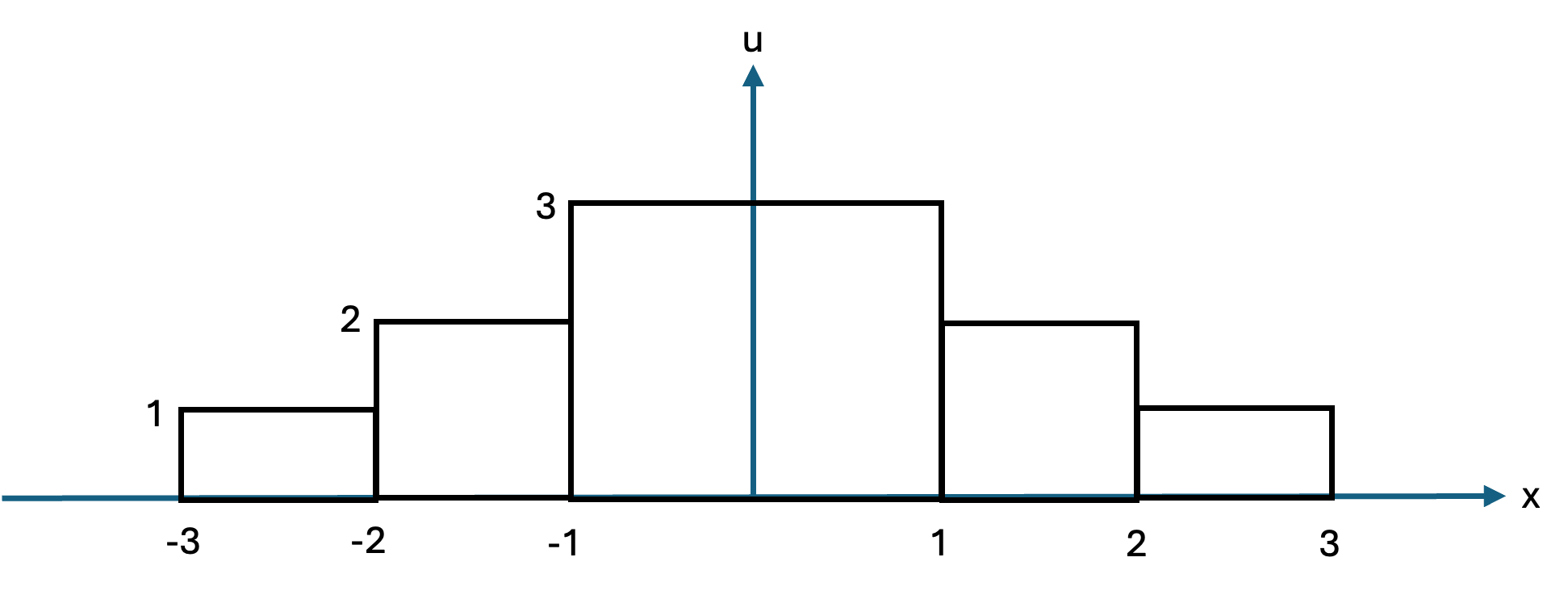
Assuming the initial velocity \(u_t(x,0)=0\), describe the solution of this problem in the \(xt\)-plane and plot the solution at \(t=4\) in the \(xu\)-plane
Solution
# Re-import libraries due to code state reset
import numpy as np
import matplotlib.pyplot as plt
import matplotlib.animation as animation
from IPython.display import HTML

# Define the piecewise function f(x)
def fa(x):
    x = np.array(x)
    result = np.zeros_like(x)
    result[(x >= -3) & (x < -2)] = 1
    result[(x > -2) & (x < -1)] = 2
    result[(x >= -1) & (x < 1)] = 1
    result[(x >= 1) & (x < 2)] = 2
    result[(x >= 2) & (x < 3)] = 1
    # result is already 0 elsewhere
    return result

def fb(x):
    x = np.array(x)
    result = np.zeros_like(x)
    result[(x >= -3) & (x < -2)] = 1
    result[(x > -2) & (x < -1)] = 2
    result[(x >= -1) & (x < 1)] = 3
    result[(x >= 1) & (x < 2)] = 2
    result[(x >= 2) & (x < 3)] = 1
    # result is already 0 elsewhere
    return result
# Create meshgrid
x = np.linspace(-10, 10, 400)
t = np.linspace(0, 6, 200)
X, T = np.meshgrid(x, t)
Ua = 0.5 *(fa(X -T) +fa(X +T))
Ub = 0.5 *(fb(X -T) +fb(X +T))
# Plot u
fig, axes = plt.subplots(2, 1, figsize=(7, 7))
cba = axes[0].pcolormesh(x, t, Ua, vmin=0, vmax=3, cmap='gray_r')
cbb = axes[1].pcolormesh(x, t, Ub, vmin=0, vmax=3, cmap='gray_r')
plt.colorbar(cba, shrink=0.9, ticks=[0, 0.5, 1, 1.5, 2, 2.5, 3], label='u')
plt.colorbar(cbb, shrink=0.9, ticks=[0, 0.5, 1, 1.5, 2, 2.5, 3], label='u')
axes[0].axhline(y=4, color="black", linestyle=":", label='$t=4$')
axes[1].axhline(y=4, color="black", linestyle=":", label='$t=4$')
# Plot characteristics
for x0 in [-3, -2, -1, 1, 2, 3]:
axes[0].plot(x0 +t, t, 'red', linestyle=':')
axes[0].plot(x0 -t, t, 'red', linestyle=':')
axes[1].plot(x0 +t, t, 'red', linestyle=':')
axes[1].plot(x0 -t, t, 'red', linestyle=':')
axes[0].set_title('Characteristic Lines and $u(x,t)$ in $x$-$t$ Plane')
axes[1].set_xlabel('x')
axes[0].set_ylabel('t')
axes[1].set_ylabel('t')
plt.legend(loc=4)
plt.tight_layout()
plt.show()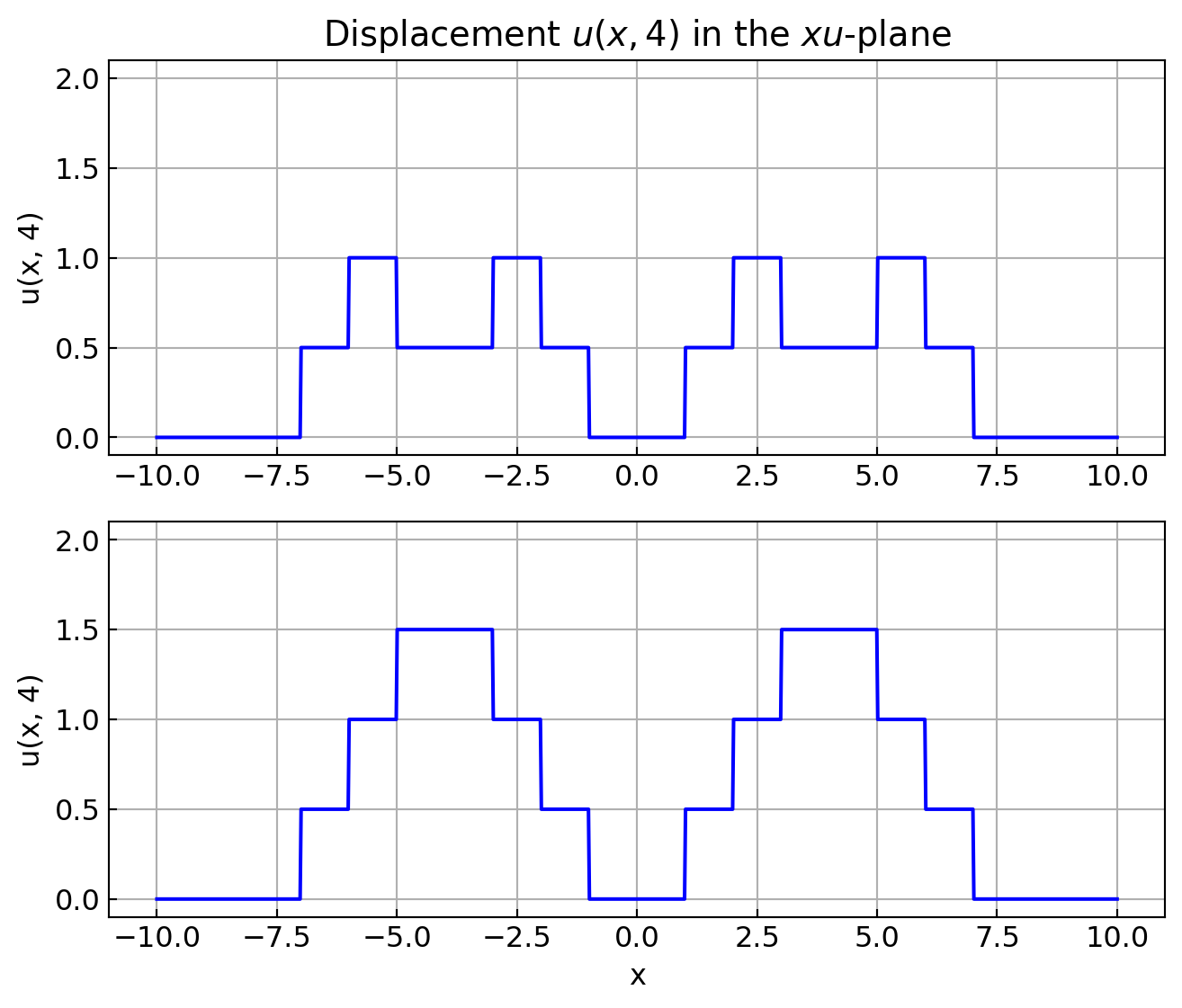
# Define u(x, t) = 1/2 [f(x -t) +f(x +t)] at t = 4

t = 4
x_vals = np.linspace(-10, 10, 1000)
ua_vals = 0.5 *(fa(x_vals -t) +fa(x_vals +t))
ub_vals = 0.5 *(fb(x_vals -t) +fb(x_vals +t))

# Plot u(x, 4)
fig, axes = plt.subplots(2, 1, figsize=(7, 6))

axes[0].plot(x_vals, ua_vals, color='blue')
axes[1].plot(x_vals, ub_vals, color='blue')

axes[0].set_title('Displacement $u(x, 4)$ in the $xu$-plane')
axes[1].set_xlabel('x')
axes[0].set_ylabel('u(x, 4)')
axes[1].set_ylabel('u(x, 4)')
axes[0].grid(True)
axes[1].grid(True)

axes[0].set_ylim([-0.1, 2.1])
axes[1].set_ylim([-0.1, 2.1])

plt.tight_layout()
plt.show()
# Create grid
x = np.linspace(-10, 10, 400)
t_vals_light = np.linspace(0, 6, 40)

# Set up the figure
fig, axes = plt.subplots(2, 1, figsize=(7, 6))

line0, = axes[0].plot([], [], lw=2)
line1, = axes[1].plot([], [], lw=2)
axes[0].set_xlim(-10, 10)
axes[1].set_xlim(-10, 10)

axes[0].set_ylim(-0.1, 3.1)
axes[1].set_ylim(-0.1, 3.1)

axes[1].set_xlabel('x')
axes[0].set_ylabel('u(x,t)')
axes[1].set_ylabel('u(x,t)')
#axes[0].set_title('Wave Propagation Over Time')

plt.close()

# Animation functions
def init():
    line0.set_data([], [])
    line1.set_data([], [])
    return line0, line1

def animate(i):
    t = t_vals_light[i]
    ua = 0.5 *(fa(x -t) +fa(x +t))
    ub = 0.5 *(fb(x -t) +fb(x +t))
    line0.set_data(x, ua)
    line1.set_data(x, ub)
    axes[0].set_title(f'Wave at t = {t:.2f}')
    return line0, line1

# Create and save animation
ani = animation.FuncAnimation(fig, animate, frames=len(t_vals_light),
                              init_func=init, blit=True, interval=400)

HTML('<center>' + ani.to_html5_video() + '</center>')\(~\)
6. \(~\) Find \(u\left( \frac{3}{8}, 3 \right)\)
\[ \begin{aligned} u_{tt} &= u_{xx}, \;\;0<x<1, \; 0 < t < \infty\\ u_x(0, t) &= 0\\ u(1, t) &= 0\\ u(x, 0) &=(1-x)^3 \\ u_t(x, 0) &= (1-x)^2 \end{aligned} \]
Solution
Method of Solution: D’Alembert’s Formula with Function Extension
Step 1: \(~\) D’Alembert Solution on the Infinite Domain
The general D’Alembert solution for the wave equation on the entire real line is:
\[u(x,t) = \frac{1}{2}\left[f(x + t) + f(x - t)\right] + \frac{1}{2} \int_{x - t}^{x + t} g(s)\, ds\]
This solution assumes that u is defined on the entire real line with no boundary conditions. To use this method on the interval \(0 < x < 1\), we extend \(f(x)\) and \(g(x)\) to the whole real line by reflecting them in such a way that the boundary conditions are satisfied
Step 2: \(~\) Extend \(f(x)\) and \(g(x)\) to the Real Line
We extend \(f(x)\) and \(g(x)\) as follows:
Boundary Conditions:
- Neumann at \(x = 0 \;\Rightarrow\;\) Extend as an even function about \(x\) = 0
- Dirichlet at \(x = 1 \;\Rightarrow\;\) Extend as an odd function about \(x = 1\)
This leads to a 2-periodic extension over \(\mathbb{R}\). The steps:
- Reflect \(f(x)\), \(g(x)\) evenly about \(x = 0\)
- Reflect them oddly about \(x = 1\)
- Periodically extend with period 4
We denote the extended functions as \(\tilde{f}(x)\), \(\tilde{g}(x)\), defined for all \(x \in \mathbb{R}\) and this pattern repeats every 4 units:
\[\tilde{f}(x + 4) = \tilde{f}(x)\]
Step 3: \(~\) Apply D’Alembert Formula
Using the extended functions, the D’Alembert solution becomes:
\[u(x,t) = \frac{1}{2} \left[\tilde{f}(x + t) + \tilde{f}(x - t)\right] + \frac{1}{2} \int_{x - t}^{x + t} \tilde{g}(s)\, ds\]
Now substitute \(x = \frac{3}{8}\), \(t = 3\):
\[u\left( \frac{3}{8}, 3 \right) = \frac{1}{2} \left[ \tilde{f}\left(\frac{3}{8} + 3\right) + \tilde{f}\left(\frac{3}{8} - 3\right) \right] + \frac{1}{2} \int_{\frac{3}{8} - 3}^{\frac{3}{8} + 3} \tilde{g}(s)\, ds\]
- Construction of \(\tilde{f}(x)\) on \([0, 4)\):
| Interval | Definition of \(\tilde{f}(x)\) | Reasoning |
|---|---|---|
| \(0 \leq x < 1\) | \((1 - x)^3\) | Original definition |
| \(1 \leq x < 2\) | \((1 - x)^3\) | Odd reflection about \(x = 1\) |
| \(2 \leq x < 3\) | \((x - 3)^3\) | Even reflection about \(x = 2\) of previous term |
| \(3 \leq x < 4\) | \((x - 3)^3\) | Odd reflection about \(x = 3\) of previous term |
- Construction of \(\tilde{g}(x)\) on \([0, 4)\):
| Interval | Definition of \(\tilde{g}(x)\) | Reasoning |
|---|---|---|
| \(0 \leq x < 1\) | \(\phantom{-}(1 - x)^2\) | Original definition |
| \(1 \leq x < 2\) | \(-(1 - x)^2\) | Odd reflection about \(x = 1\) |
| \(2 \leq x < 3\) | \(-(x - 3)^2\) | Even reflection about \(x = 2\) of previous term |
| \(3 \leq x < 4\) | \(\phantom{-}(x - 3)^2\) | Odd reflection about \(x = 3\) of previous term |
import numpy as np
import matplotlib.pyplot as plt

def tilde_fg(x):
    x = np.array(x)
    f = np.zeros_like(x)
    g = np.zeros_like(x)

    # (0, 1): original
    mask1 = (0 <= x) & (x < 1)
    f[mask1] = (1 -x[mask1])**3
    g[mask1] = (1 -x[mask1])**2

    # (1, 2): odd reflection about x = 1
    mask2 = (1 <= x) & (x < 2)
    f[mask2] = (1 -x[mask2])**3
    g[mask2] = -(1 -x[mask2])**2

    # (2, 3): even reflection about x = 2
    mask3 = (2 <= x) & (x < 3)
    f[mask3] = (x[mask3] -3)**3  # no sign change
    g[mask3] = -(x[mask3] -3)**2

    # (3, 4): odd reflection about x = 3
    mask4 = (3 <= x) & (x <= 4)
    f[mask4] = (x[mask4] -3)**3
    g[mask4] = (x[mask4] -3)**2

    return f, g

# Domain
x_vals = np.linspace(0, 4, 1000)
f_vals, g_vals = tilde_fg(x_vals)

# Plot
plt.figure(figsize=(6, 4))
plt.plot(x_vals, f_vals, color='red', label=r'$\tilde{f}$')
plt.plot(x_vals, g_vals, color='blue', label=r'$\tilde{g}$')

plt.title(r'$\tilde{f}(x), \tilde{g}(x)$ on $[0, 4)$')
plt.xlabel('x')
plt.ylabel(r'$\tilde{f}(x), \tilde{g}(x)$')
plt.legend()
plt.grid(True)
plt.tight_layout()
plt.show()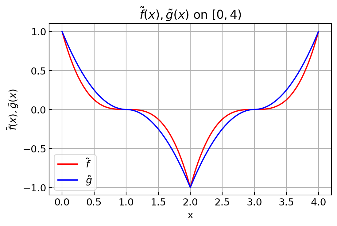
Step 4: \(~\) Evaluate \(\tilde{f}(x \pm t)\)
\[x = \frac{3}{8} = 0.375,\quad t = 3 \Rightarrow x + t = 3.375,\quad x - t = -2.625\]
Using 4-periodicity:
- \(3.375 \mod 4 = 3.375\)
- \(-2.625 \mod 4 = 1.375\)
Thus:
- \(\tilde{f}(3.375) = (3.375 - 3)^3 = (0.375)^3 = \frac{27}{512}\)
- \(\tilde{f}(1.375) = (1 -1.375)^3 = - (0.375)^3 = -\frac{27}{512}\)
So the average is:
\[\frac{1}{2} \left[ \tilde{f}(3.375) + \tilde{f}(-2.625) \right] = \frac{1}{2} \left( \frac{27}{512} - \frac{27}{512} \right) = 0\]
Step 5: \(~\) Evaluate the Integral Term
We now compute:
\[\int_{-2.625}^{3.375} \tilde{g}(s)\, ds = \underbrace{\int_{-2.625}^{-2} \tilde{g}(s)\, ds}_{A} +\underbrace{\int_{-2}^{2} \tilde{g}(s)\, ds}_{0} +\underbrace{\int_{2}^{3.375} \tilde{g}(s)\, ds}_{B}\]
We computed the tails:
\(\displaystyle A = \int_{-2.625}^{-2} \tilde{g}(s)\, ds = -\int_{1.375}^{2} (s - 1)^2 ds = \boxed{-\frac{485}{1536}}\)
\(\displaystyle B = \int_{2}^{3.375} \tilde{g}(s)\, ds\)
We split this into two parts, because the definition of \(\tilde{g}(s)\) changes at \(s = 3\):
On \([2, 3)\): \(\tilde{g}(s) = (3 - s)^2\)
\[\int_{2}^{3} (3 - s)^2 ds = \int_1^0 u^2 (-du) = \int_0^1 u^2 du = \left[\frac{u^3}{3}\right]_0^1 = \frac{1}{3}\]
On \([3, 3.375]\): \(\tilde{g}(s) = -(s - 3)^2\)
\[\int_{3}^{3.375} - (s - 3)^2 ds = - \int_0^{3/8} v^2 dv = - \left[\frac{v^3}{3}\right]_0^{3/8} = - \frac{(3/8)^3}{3} = - \frac{27}{1536}\]
So:
\[\int_{2}^{3.375} \tilde{g}(s)\, ds = \frac{1}{3} - \frac{27}{1536} = \frac{512 - 27}{1536} = \boxed{\frac{485}{1536}}\]
Final Answer:
Recall that from the previous step:
\[\frac{1}{2} [\tilde{f}(x+t) + \tilde{f}(x - t)] = 0 \quad\text{and}\quad \text{(integral term)} = 0\]
\[\boxed{u\left( \frac{3}{8}, 3 \right) = 0}\]
\(~\)
7. \(~\) Suppose the vibration of a string is described by \(u_{tt}=u_{xx}\) and has an initial displacement as given by the following diagram:
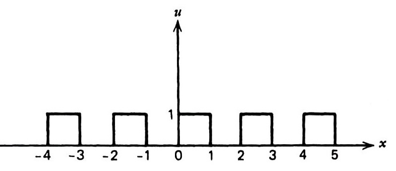
Assuming the initial velocity \(u_t(x,0)=0\), describe the solution of this problem in the \(xt\)-plane
\(~\)
8. \(~\) Consider the one-dimensional wave equation on the interval \(0 < x < L\):
\[ \begin{aligned} u_{tt}(x,t) &= c^2 u_{xx}(x,t), & 0 < x < L,\\[4pt] u(0,t) &= 0, \; u(L,t) = 0, & t > 0,\\[4pt] u(x,0) &= u_0(x), \; u_t(x,0) = v_0(x), & 0 \le x \le L \end{aligned} \]
(a) Write down the eigenfunctions and eigenvalues for this boundary-value problem
(b) Using separation of variables, provide explicit expressions for the solution in terms of \(u_0\) and \(v_0\)
Solution
(a) Eigenfunctions and Eigenvalues
Solve \(X''+\lambda X=0\) with \(X(0)=0\) and \(X(L)=0\). Nontrivial solutions occur when \[\lambda_n = \left(\frac{n\pi}{L}\right)^2, \quad n=1,2,3,\dots\] and the eigenfunctions are \[\phi_n(x)=\sin\frac{n\pi x}{L}\]
(b)-1 Series representation
The general solution is \[u(x,t)=\sum_{n=1}^{\infty}\Big(A_n\cos\frac{cn\pi t}{L}+B_n\sin\frac{cn\pi t}{L}\Big)\sin\frac{n\pi x}{L}\] This follows by separation of variables: \(u(x,t)=X(x)T(t)\) leads to the spatial eigenfunctions above, and \(T(t)\) solves \(T''+c^2\lambda_n T=0\)
(b)-2 Coefficients \(A_n\) and \(B_n\)
Using orthogonality: \[A_n = \frac{2}{L}\int_0^L u_0(x)\sin\frac{n\pi x}{L}\,dx\] \[B_n = \frac{2}{cn\pi}\int_0^L v_0(x)\sin\frac{n\pi x}{L}\,dx\]