import numpy as np

print("numpy: ", np.__version__)
numpy: 2.3.1\(~\)
![]()
\(~\)
import numpy as np
print("numpy: ", np.__version__)numpy: 2.3.1show_array()show_array_aggregation()data = np.array([[1, 2], [3, 4], [5, 6]])
dataarray([[1, 2],
[3, 4],
[5, 6]])type(data)numpy.ndarraydata.ndim2data.shape(3, 2)data.size6data.dtypedtype('int64')data.nbytes48d0 = np.array([1, 2, 3], dtype=int)
d0array([1, 2, 3])d1 = np.array([1, 2, 3], dtype=float)
d1array([1., 2., 3.])d2 = np.array([1, 2, 3], dtype=complex)
d2array([1.+0.j, 2.+0.j, 3.+0.j])data = np.array([1, 2, 3], dtype=float)
dataarray([1., 2., 3.])data = np.array(data, dtype=int)
dataarray([1, 2, 3])data = np.array([1.6, 2, 3], dtype=float)
data.astype(int)array([1, 2, 3])d1 = np.array([1, 2, 3], dtype=float)
d2 = np.array([1, 2, 3], dtype=complex)d1 + d2array([2.+0.j, 4.+0.j, 6.+0.j])(d1 + d2).dtypedtype('complex128')np.sqrt(np.array([-1, 0, 1]))/var/folders/4x/8kn2nym12cn7x7qmg_6s4b8h0000gn/T/ipykernel_76845/208196152.py:1: RuntimeWarning: invalid value encountered in sqrt
np.sqrt(np.array([-1, 0, 1]))array([nan, 0., 1.])np.sqrt(np.array([-1, 0, 1], dtype=complex))array([0.+1.j, 0.+0.j, 1.+0.j])data = np.array([1, 2, 3], dtype=complex)
dataarray([1.+0.j, 2.+0.j, 3.+0.j])data.realarray([1., 2., 3.])data.imagarray([0., 0., 0.])np.real(data)array([1., 2., 3.])np.imag(data)array([0., 0., 0.])Multidimensional arrays are stored as contiguous data in memory. \(~\)Consider the case of a two-dimensional array, \(~\)containing rows and columns: \(~\)One possible way to store this array as a consecutive sequence of values is to store the rows after each other, and another equally valid approach is to store the columns one after another
The former is called row-major format and the latter is column-major format. Whether to use row-major or column-major is a matter of conventions, and the row-major format is used for example in the C programming language, and Fortran uses the column-major format
A numpy array can be specified to be stored in row-major format, using the keyword argument order='C', and column-major format, using the keyword argument order='F', when the array is created or reshaped. The default format is row-major
In general, the numpy array attribute ndarray.strides defines exactly how this mapping is done. The strides attribute is a tuple of the same length as the number of axes (dimensions) of the array. Each value in strides is the factor by which the index for the corresponding axis is multiplied when calculating the memory offset (in bytes) for a given index expression
data = np.array([[1, 2, 3], [4, 5, 6]], dtype=np.int32)
data
array([[1, 2, 3],
[4, 5, 6]], dtype=int32)data.strides(12, 4)data = np.array([[1, 2, 3], [4, 5, 6]], dtype=np.int32, order='F')
dataarray([[1, 2, 3],
[4, 5, 6]], dtype=int32)data.strides(4, 8)data = np.array([1, 2, 3, 4])
data.ndim, data.shape(1, (4,))data = np.array(((1, 2), (3, 4)))
data.ndim, data.shape(2, (2, 2))np.zeros((2, 3))array([[0., 0., 0.],
[0., 0., 0.]])data = np.ones(4)
data, data.dtype(array([1., 1., 1., 1.]), dtype('float64'))5.4 * np.ones(10)array([5.4, 5.4, 5.4, 5.4, 5.4, 5.4, 5.4, 5.4, 5.4, 5.4])np.full(10, 5.4) # slightly more efficientarray([5.4, 5.4, 5.4, 5.4, 5.4, 5.4, 5.4, 5.4, 5.4, 5.4])x1 = np.empty(5)
x1.fill(3.0)
x1array([3., 3., 3., 3., 3.])np.arange(0, 11, 1)array([ 0, 1, 2, 3, 4, 5, 6, 7, 8, 9, 10])np.linspace(0, 10, 11) # generally recommendedarray([ 0., 1., 2., 3., 4., 5., 6., 7., 8., 9., 10.])np.logspace(0, 2, 10) # 5 data points between 10**0=1 to 10**2=100array([ 1. , 1.66810054, 2.7825594 , 4.64158883,
7.74263683, 12.91549665, 21.5443469 , 35.93813664,
59.94842503, 100. ])x = np.array([-1, 0, 1])
y = np.array([-2, 0, 2])
X, Y = np.meshgrid(x, y)Xarray([[-1, 0, 1],
[-1, 0, 1],
[-1, 0, 1]])Yarray([[-2, -2, -2],
[ 0, 0, 0],
[ 2, 2, 2]])Z = (X + Y)**2
Zarray([[9, 4, 1],
[1, 0, 1],
[1, 4, 9]])np.empty(3, dtype=float)array([0., 0., 0.])def f(x):
y = np.ones_like(x) # compute with x and y
return y
x = np.array([[1, 2, 3], [4, 5, 6]])
y = f(x)
yarray([[1, 1, 1],
[1, 1, 1]])np.identity(4)array([[1., 0., 0., 0.],
[0., 1., 0., 0.],
[0., 0., 1., 0.],
[0., 0., 0., 1.]])np.eye(4, k=1)array([[0., 1., 0., 0.],
[0., 0., 1., 0.],
[0., 0., 0., 1.],
[0., 0., 0., 0.]])np.eye(4, k=-1)array([[0., 0., 0., 0.],
[1., 0., 0., 0.],
[0., 1., 0., 0.],
[0., 0., 1., 0.]])np.diag(np.arange(0, 20, 5))array([[ 0, 0, 0, 0],
[ 0, 5, 0, 0],
[ 0, 0, 10, 0],
[ 0, 0, 0, 15]])a = np.arange(0, 11)
aarray([ 0, 1, 2, 3, 4, 5, 6, 7, 8, 9, 10])a[0]np.int64(0)a[-1]np.int64(10)a[4]np.int64(4)a[1:-1]array([1, 2, 3, 4, 5, 6, 7, 8, 9])a[1:-1:2]array([1, 3, 5, 7, 9])a[:5]array([0, 1, 2, 3, 4])a[-5:]array([ 6, 7, 8, 9, 10])a[::-2]array([10, 8, 6, 4, 2, 0])f = lambda m, n: n + 10*m# please search for numpy.fromfunction at google
A = np.fromfunction(f, (6, 6), dtype=int)
A array([[ 0, 1, 2, 3, 4, 5],
[10, 11, 12, 13, 14, 15],
[20, 21, 22, 23, 24, 25],
[30, 31, 32, 33, 34, 35],
[40, 41, 42, 43, 44, 45],
[50, 51, 52, 53, 54, 55]])A[:, 1] # the second columnarray([ 1, 11, 21, 31, 41, 51])A[1, :] # the second rowarray([10, 11, 12, 13, 14, 15])A[:3, :3]array([[ 0, 1, 2],
[10, 11, 12],
[20, 21, 22]])A[3:, :3]array([[30, 31, 32],
[40, 41, 42],
[50, 51, 52]])A[::2, ::2]array([[ 0, 2, 4],
[20, 22, 24],
[40, 42, 44]])A[1::2, 1::3]array([[11, 14],
[31, 34],
[51, 54]])Subarrays that are extracted from arrays using slice operations are alternative views of the same underlying array data. That is, \(~\)they are arrays that refer to the same data in memory as the original array, \(~\)but with a different strides configuration
When elements in a view are assigned new values, \(~\)the values of the original array are therefore also updated. For example,
B = A[1:5, 1:5]
B
array([[11, 12, 13, 14],
[21, 22, 23, 24],
[31, 32, 33, 34],
[41, 42, 43, 44]])B[:, :] = 0
Aarray([[ 0, 1, 2, 3, 4, 5],
[10, 0, 0, 0, 0, 15],
[20, 0, 0, 0, 0, 25],
[30, 0, 0, 0, 0, 35],
[40, 0, 0, 0, 0, 45],
[50, 51, 52, 53, 54, 55]])copy method of the ndarray instanceC = B[1:3, 1:3].copy()
Carray([[0, 0],
[0, 0]])C[:, :] = 1
Carray([[1, 1],
[1, 1]])Barray([[0, 0, 0, 0],
[0, 0, 0, 0],
[0, 0, 0, 0],
[0, 0, 0, 0]])A = np.linspace(0, 1, 11)
Aarray([0. , 0.1, 0.2, 0.3, 0.4, 0.5, 0.6, 0.7, 0.8, 0.9, 1. ])A[np.array([0, 2, 4])]array([0. , 0.2, 0.4])A[[0, 2, 4]]array([0. , 0.2, 0.4])A > 0.5array([False, False, False, False, False, False, True, True, True,
True, True])A[A > 0.5]array([0.6, 0.7, 0.8, 0.9, 1. ])A = np.arange(10)
indices = [2, 4, 6]B = A[indices]B[0] = -1
Aarray([0, 1, 2, 3, 4, 5, 6, 7, 8, 9])A[indices] = -1
Aarray([ 0, 1, -1, 3, -1, 5, -1, 7, 8, 9])A = np.arange(10)B = A[A > 5]B[0] = -1
Aarray([0, 1, 2, 3, 4, 5, 6, 7, 8, 9])A[A > 5] = -1
Aarray([ 0, 1, 2, 3, 4, 5, -1, -1, -1, -1])show_array((4, 4), ':, :')
show_array((4, 4), '0')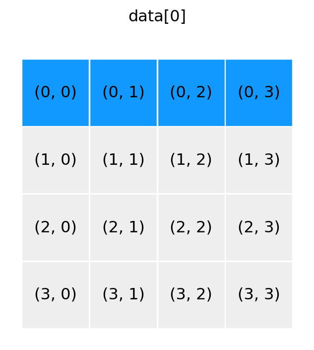
show_array((4, 4), '1, :')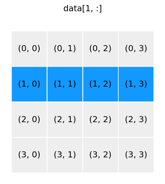
show_array((4, 4), ':, 2')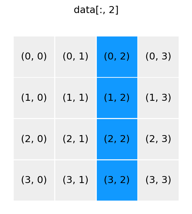
show_array((4, 4), '0:2, 0:2')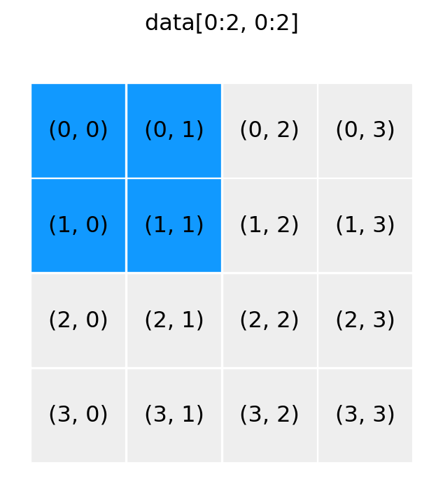
show_array((4, 4), '0:2, 2:4')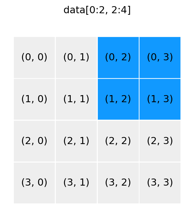
show_array((4, 4), '::2, ::2')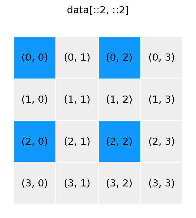
show_array((4, 4), '1::2, 1::2')
show_array((4, 4), ':, [0, 3]')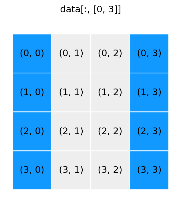
show_array((4, 4), '[1, 3], [0, 3]')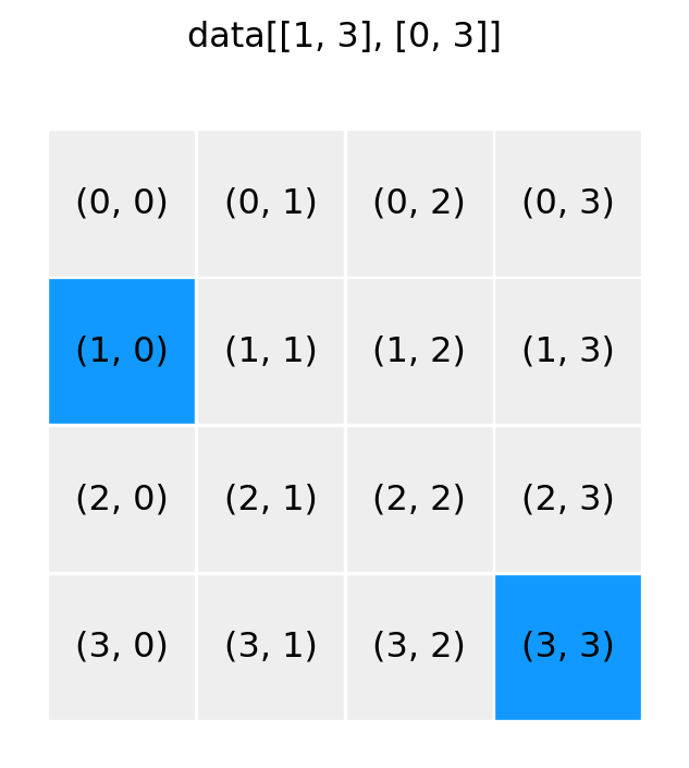
show_array((4, 4), ':, [False, True, True, False]')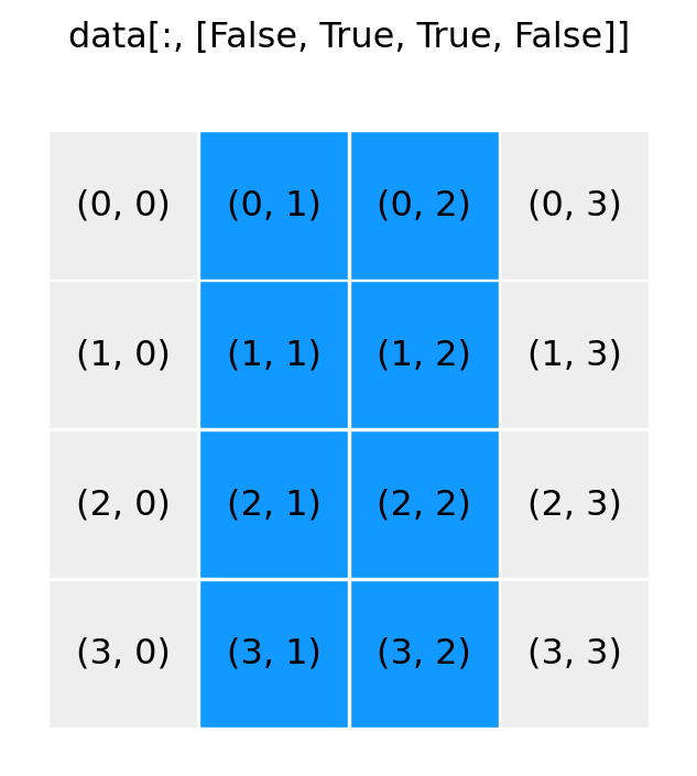
show_array((4, 4), '1:3, [False, True, True, False]')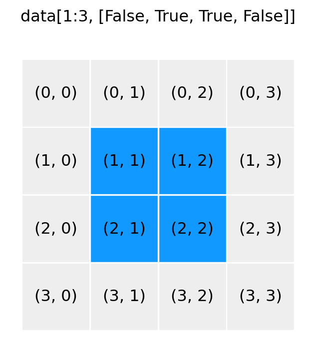
data = np.array([[1, 2], [3, 4]])
data1 = np.reshape(data, (1, 4))
data1
array([[1, 2, 3, 4]])data1[0, 1] = -1
dataarray([[ 1, -1],
[ 3, 4]])data2 = data.reshape(4)
data2array([ 1, -1, 3, 4])data2[1] = -2
dataarray([[ 1, -2],
[ 3, 4]])data = np.array([[1, 2], [3, 4]])
data1 = np.ravel(data)
data1array([1, 2, 3, 4])data1[0] = -1
dataarray([[-1, 2],
[ 3, 4]])ndarray method flatten perform the same function, \(~\)but returns a copy instead of a viewdata2 = data.flatten()
data2array([-1, 2, 3, 4])data2[0] = -2
dataarray([[-1, 2],
[ 3, 4]])data = np.arange(0, 5)
data.shape(5,)column = data[:, np.newaxis]
columnarray([[0],
[1],
[2],
[3],
[4]])column.shape(5, 1)row = data[np.newaxis, :]
rowarray([[0, 1, 2, 3, 4]])row.shape(1, 5)row[0, 0] = -1
dataarray([-1, 1, 2, 3, 4])np.expand_dims(data, axis=1) array([[-1],
[ 1],
[ 2],
[ 3],
[ 4]])row = np.expand_dims(data, axis=0)
rowarray([[-1, 1, 2, 3, 4]])row[0, 0] = 0
dataarray([0, 1, 2, 3, 4])data = np.arange(5)
dataarray([0, 1, 2, 3, 4])np.vstack((data, data, data))array([[0, 1, 2, 3, 4],
[0, 1, 2, 3, 4],
[0, 1, 2, 3, 4]])np.hstack((data, data, data))array([0, 1, 2, 3, 4, 0, 1, 2, 3, 4, 0, 1, 2, 3, 4])data = data[:, np.newaxis]
data.shape(5, 1)np.hstack((data, data, data))array([[0, 0, 0],
[1, 1, 1],
[2, 2, 2],
[3, 3, 3],
[4, 4, 4]])data1 = np.array([[1, 2], [3, 4]])
data2 = np.array([[5, 6]])np.concatenate((data1, data2), axis=0)array([[1, 2],
[3, 4],
[5, 6]])np.concatenate((data1, data2.T), axis=1)array([[1, 2, 5],
[3, 4, 6]])x = np.array([[1, 2], [3, 4]])
y = np.array([[5, 6], [7, 8]])x + yarray([[ 6, 8],
[10, 12]])y - xarray([[4, 4],
[4, 4]])x * yarray([[ 5, 12],
[21, 32]])y / xarray([[5. , 3. ],
[2.33333333, 2. ]])x * 2array([[2, 4],
[6, 8]])2**xarray([[ 2, 4],
[ 8, 16]])y / 2array([[2.5, 3. ],
[3.5, 4. ]])(y / 2).dtypedtype('float64')a = np.array([[11, 12, 13], [21, 22, 23], [31, 32, 33]])
b = np.array([[1, 2, 3]])a + barray([[12, 14, 16],
[22, 24, 26],
[32, 34, 36]])show_array_broadcasting(a, b)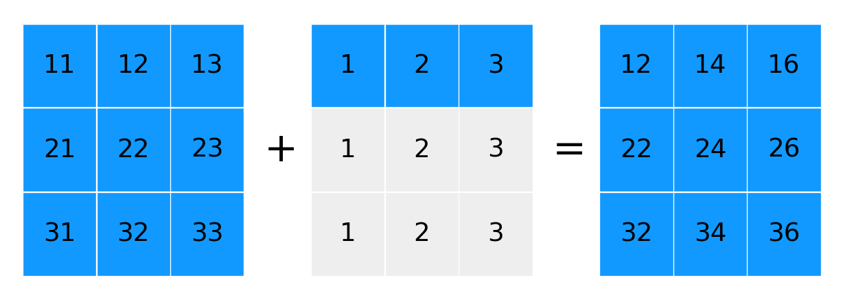
a + b.Tarray([[12, 13, 14],
[23, 24, 25],
[34, 35, 36]])show_array_broadcasting(a, b.T)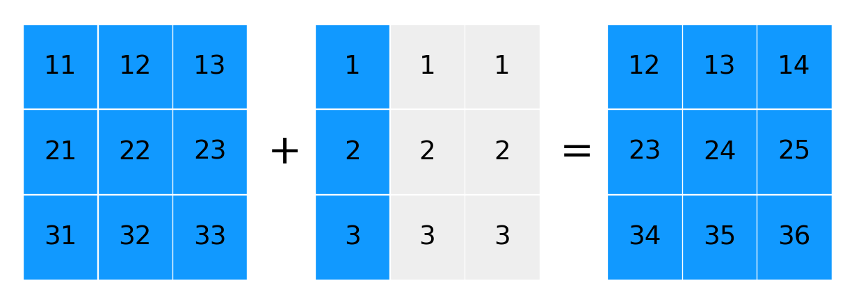
x = np.array([1, 2, 3, 4]).reshape(2, 2)
x.shape
(2, 2)z = np.array([[2, 4]])
z.shape(1, 2)x / zarray([[0.5, 0.5],
[1.5, 1. ]])zz = np.vstack((z, z))
zzarray([[2, 4],
[2, 4]])x / zzarray([[0.5, 0.5],
[1.5, 1. ]])z = np.array([[2], [4]])
z.shape(2, 1)x / zarray([[0.5 , 1. ],
[0.75, 1. ]])zz = np.concatenate([z, z], axis=1)
zzarray([[2, 2],
[4, 4]])x / zzarray([[0.5 , 1. ],
[0.75, 1. ]])x = z = np.array([1, 2, 3, 4])
y = np.array([5, 6, 7, 8])
x = x + y # x is reassigned to a new arrayx, z(array([ 6, 8, 10, 12]), array([1, 2, 3, 4]))x = z = np.array([1, 2, 3, 4])
y = np.array([5, 6, 7, 8])
x += y # the values of array x are updated in placex, z(array([ 6, 8, 10, 12]), array([ 6, 8, 10, 12]))x = np.linspace(-1, 1, 11)
xarray([-1. , -0.8, -0.6, -0.4, -0.2, 0. , 0.2, 0.4, 0.6, 0.8, 1. ])y = np.sin(np.pi * x)np.round(y, decimals=4)array([-0. , -0.5878, -0.9511, -0.9511, -0.5878, 0. , 0.5878,
0.9511, 0.9511, 0.5878, 0. ])np.add(np.sin(x)**2, np.cos(x)**2)array([1., 1., 1., 1., 1., 1., 1., 1., 1., 1., 1.])np.sin(x)**2 + np.cos(x)**2array([1., 1., 1., 1., 1., 1., 1., 1., 1., 1., 1.])def heaviside(x):
return 1 if x > 0 else 0heaviside(-1)0heaviside(1.5)1```{python}
x = np.linspace(-5, 5, 11)
heaviside(x)
```
ValueError
1 x = np.linspace(-5, 5, 11)
----> 2 heaviside(x)
1 def heaviside(x):
----> 2 return 1 if x > 0 else 0
ValueError: The truth value of an array with more than
one element is ambiguous. Use a.any() or a.all()heaviside = np.vectorize(heaviside)
heaviside(x)array([0, 0, 0, 0, 0, 0, 1, 1, 1, 1, 1])def heaviside(x): # much better way
return 1 * (x > 0)
heaviside(x)array([0, 0, 0, 0, 0, 0, 1, 1, 1, 1, 1])data = np.random.normal(size=(15, 15)) np.mean(data)np.float64(-0.041673140354896374)data.mean()np.float64(-0.041673140354896374)data = np.random.normal(size=(5, 10, 15))data.sum(axis=0).shape(10, 15)data.sum(axis=(0, 2)).shape(10,)data.sum()np.float64(18.68747786875952)data = np.arange(9).reshape(3, 3)
dataarray([[0, 1, 2],
[3, 4, 5],
[6, 7, 8]])data.sum()np.int64(36)show_array_aggregation(data, None)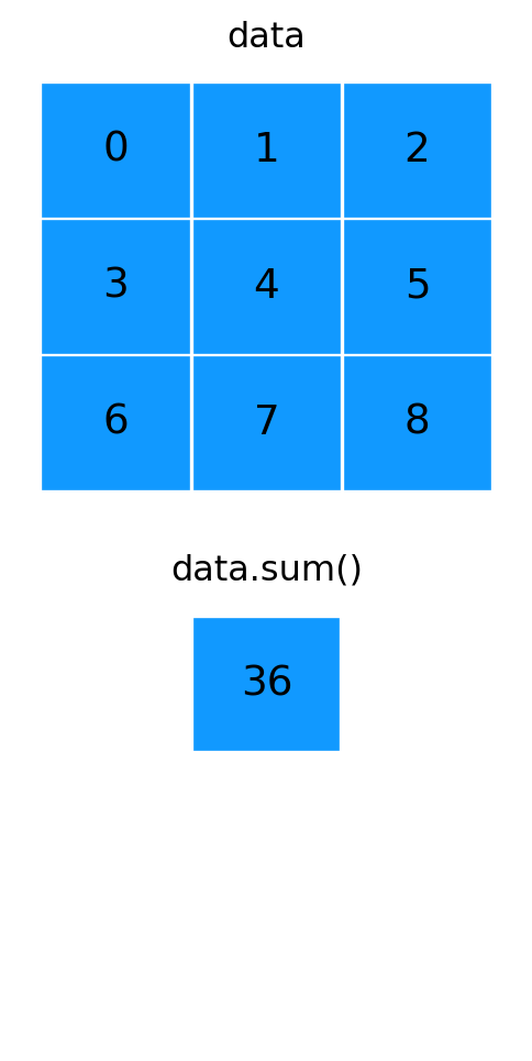
data.sum(axis=0)array([ 9, 12, 15])show_array_aggregation(data, 0)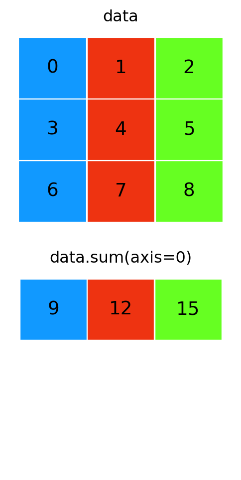
data.sum(axis=1)array([ 3, 12, 21])show_array_aggregation(data, 1)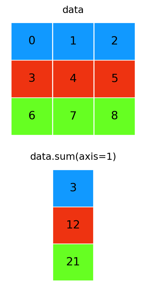
a = np.array([1, 2, 3, 4])
b = np.array([4, 3, 2, 1])
a < barray([ True, True, False, False])np.all(a < b)np.False_np.any(a < b)np.True_x = np.array([-2, -1, 0, 1, 2])x > 0array([False, False, False, True, True])1 * (x > 0)array([0, 0, 0, 1, 1])x * (x > 0)array([0, 0, 0, 1, 2])def pulse(x, position, height, width):
return height * (x >= position) * (x <= (position + width)) x = np.linspace(-5, 5, 31)pulse(x, position=-2, height=1, width=5)array([0, 0, 0, 0, 0, 0, 0, 0, 0, 1, 1, 1, 1, 1, 1, 1, 1, 1, 1, 1, 1, 1,
1, 1, 1, 0, 0, 0, 0, 0, 0])pulse(x, position=1, height=2, width=2)array([0, 0, 0, 0, 0, 0, 0, 0, 0, 0, 0, 0, 0, 0, 0, 0, 0, 0, 2, 2, 2, 2,
2, 2, 2, 0, 0, 0, 0, 0, 0])x = np.linspace(-4, 4, 9)
xarray([-4., -3., -2., -1., 0., 1., 2., 3., 4.])np.where(x < 0, x**2, x**3)array([16., 9., 4., 1., 0., 1., 8., 27., 64.])np.select([x < -1, x < 2, x>= 2], [x**2, x**3, x**4])array([ 16., 9., 4., -1., 0., 1., 16., 81., 256.])np.choose([0, 0, 0, 1, 1, 1, 2, 2, 2], [x**2, x**3, x**4])array([ 16., 9., 4., -1., 0., 1., 16., 81., 256.])x[np.abs(x) > 2]array([-4., -3., 3., 4.])a = np.unique([1, 2, 3, 3])
aarray([1, 2, 3])b = np.unique([2, 3, 4, 4, 5, 6, 5])
barray([2, 3, 4, 5, 6])np.in1d(a, b)/var/folders/4x/8kn2nym12cn7x7qmg_6s4b8h0000gn/T/ipykernel_76845/924698060.py:1: DeprecationWarning: `in1d` is deprecated. Use `np.isin` instead.
np.in1d(a, b)array([False, True, True])1 in a, 1 in b(True, False)np.all(np.in1d(a, b)) # to test if a is a subset of b/var/folders/4x/8kn2nym12cn7x7qmg_6s4b8h0000gn/T/ipykernel_76845/423008062.py:1: DeprecationWarning: `in1d` is deprecated. Use `np.isin` instead.
np.all(np.in1d(a, b)) # to test if a is a subset of bnp.False_np.union1d(a, b)array([1, 2, 3, 4, 5, 6])np.intersect1d(a, b)array([2, 3])np.setdiff1d(a, b)array([1])np.setdiff1d(b, a)array([4, 5, 6])data = np.arange(9).reshape(3, 3)
dataarray([[0, 1, 2],
[3, 4, 5],
[6, 7, 8]])np.transpose(data)array([[0, 3, 6],
[1, 4, 7],
[2, 5, 8]])data = np.random.randn(1, 2, 3, 4, 5)data.shape(1, 2, 3, 4, 5)data.T.shape(5, 4, 3, 2, 1)A = np.arange(1, 7).reshape(2, 3)
Aarray([[1, 2, 3],
[4, 5, 6]])B = np.arange(1, 7).reshape(3, 2)
Barray([[1, 2],
[3, 4],
[5, 6]])np.dot(A, B)array([[22, 28],
[49, 64]])np.dot(B, A)array([[ 9, 12, 15],
[19, 26, 33],
[29, 40, 51]])A @ B # python 3.5 abovearray([[22, 28],
[49, 64]])B @ Aarray([[ 9, 12, 15],
[19, 26, 33],
[29, 40, 51]])A = np.arange(9).reshape(3, 3)
Aarray([[0, 1, 2],
[3, 4, 5],
[6, 7, 8]])x = np.arange(3)
xarray([0, 1, 2])np.dot(A, x)array([ 5, 14, 23])A.dot(x)array([ 5, 14, 23])A @ xarray([ 5, 14, 23])A = np.random.rand(3, 3)
B = np.random.rand(3, 3)Ap = np.dot(B, np.dot(A, np.linalg.inv(B)))Ap = B.dot(A.dot(np.linalg.inv(B)))B @ A @ np.linalg.inv(B)array([[-2.37625054, 0.83934428, 4.20566574],
[-0.53237348, 0.16362199, 4.63972309],
[-2.04694973, 0.71992986, 2.77055746]])np.inner(x, x)np.int64(5)np.dot(x, x)np.int64(5)y = x[:, np.newaxis]
yarray([[0],
[1],
[2]])np.dot(y.T, y)array([[5]])\[\begin{pmatrix} a_0 b_0 & a_0b_1 & \cdots & a_0 b_N \\ a_1 b_0 & \cdots & \cdots & a_1 b_N \\ \vdots & \ddots & & \vdots \\ a_M b_0 & & \ddots & a_M b_N \\ \end{pmatrix} \]
x = np.array([1, 2, 3])np.outer(x, x)array([[1, 2, 3],
[2, 4, 6],
[3, 6, 9]])np.kron(x, x)array([1, 2, 3, 2, 4, 6, 3, 6, 9])np.kron(x[:, np.newaxis], x[np.newaxis, :])array([[1, 2, 3],
[2, 4, 6],
[3, 6, 9]])np.kron(np.ones((2, 2)), np.identity(2))array([[1., 0., 1., 0.],
[0., 1., 0., 1.],
[1., 0., 1., 0.],
[0., 1., 0., 1.]])np.kron(np.identity(2), np.ones((2, 2)))array([[1., 1., 0., 0.],
[1., 1., 0., 0.],
[0., 0., 1., 1.],
[0., 0., 1., 1.]])x = np.array([1, 2, 3, 4])
y = np.array([5, 6, 7, 8])np.einsum("n,n", x, y)np.int64(70)np.inner(x, y)np.int64(70)A = np.arange(9).reshape(3, 3)
B = A.Tnp.einsum("mk,kn", A, B)array([[ 5, 14, 23],
[ 14, 50, 86],
[ 23, 86, 149]])np.all(np.einsum("mk,kn", A, B) == np.dot(A, B))np.True_