Notice that the independent variable \(t\) does not appear explicitly on the right-hand side of each differential equation
Second-Order DE as a System
Any second-order differential equation \(x''=g(x,x')\) can be written as an autonomous system. If we let \(y=x'\), the second-order differential equation becomes the system of two first-order equations
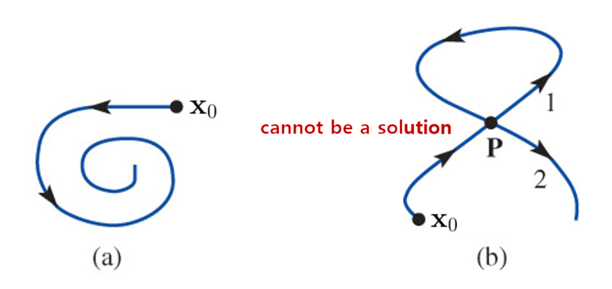
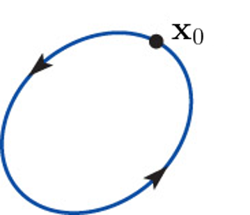
If \(P\), \(Q\), and the first-order partial derivatives \(\partial P/\partial x\), \(\partial P/\partial y\), \(\partial Q/\partial x\), and \(\partial Q/\partial y\) are continuous in a region \(R\) of the plane, then a solution to the plane autonomous system that satisfies \(\mathbf{x}(0)=\mathbf{x}_0\) is unique and one of three basic types:
A constant solution, \(\mathbf{x}(t)=\mathbf{x}_0\) for all \(t\). A constant solution is called a critical or stationary point
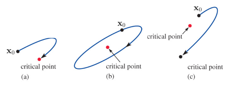
If \(\mathbf{x}_1\) is a critical point of a plane autonomous system and \(\mathbf{x}=\mathbf{x}(t)\) is a solution satisfying \(\mathbf{x}(0)=\mathbf{x}_0\), when \(\mathbf{x}_0\) is placed near \(\mathbf{x}_1\)
It may return to the critical point
It may remain close to the critical point without returning
It may move away from the critical point
Stability Analysis
A careful geometric analysis of the solutions to the linear plane autonomous system
in terms of the eigenvalues and eigenvectors of the coefficient matrix
\[\mathbf{A}=
\begin{pmatrix}
a & b\\
c & d
\end{pmatrix}
\]
drives the stabilty analysis
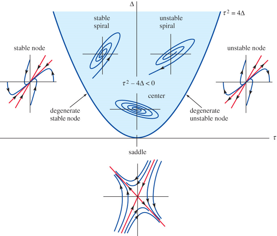
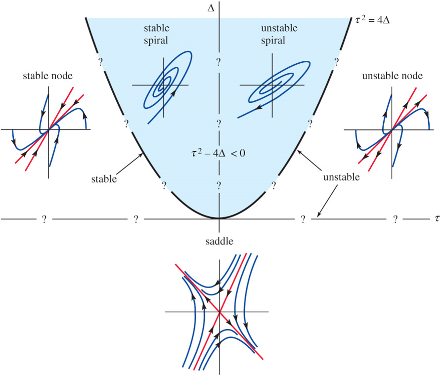
To ensure that \(\mathbf{x}_0=(0,\,0)\) is the only critical point, we will assume that the determinant \(\Delta = ad -bc \neq 0\). If \(\tau = a + d\) is the trace of matrix \(\mathbf{A}\), then the characteristic equation, \(\mathrm{det}(\mathbf{A} -\lambda\mathbf{I})=0,\) can be rewritten as
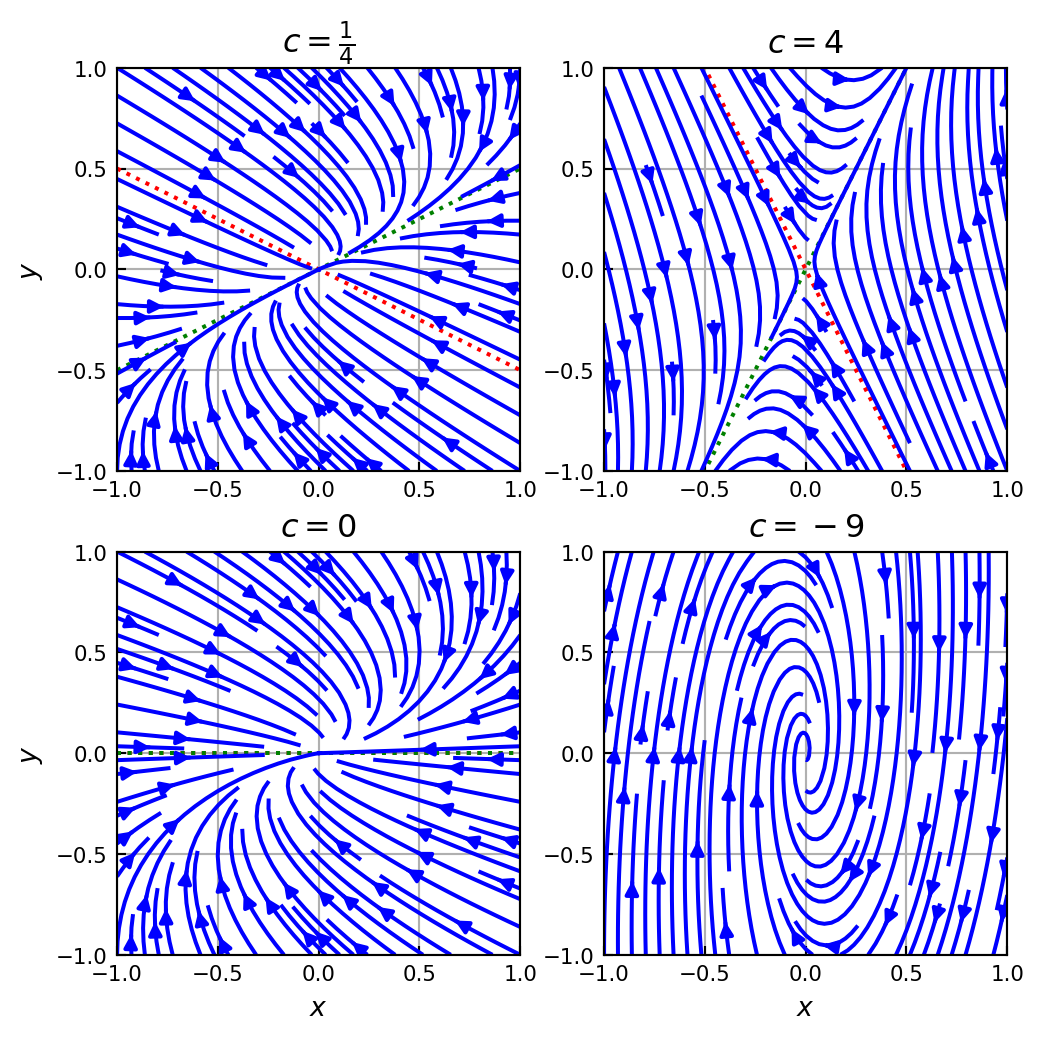
in terms of \(c\), and use a numerical solver to discover the shapes of solutions corresponding to the cases \(c=\frac{1}{4}\), \(4\), \(0\), and \(-9\). \(\mathbf{A}\) has trace \(\tau=-2\) and determinant \(\Delta=1 -c\), and so the eigenvalues are
\[ \lambda =-1 \pm \sqrt{c} \]
The nature of the eigenvalues is therefore determined by the value of \(c\)
import numpy as npimport sympy as spsp.init_printing(use_unicode=True)c = sp.Symbol('c')A = sp.Matrix([[-1, 1], [c, -1]])A.eigenvects()
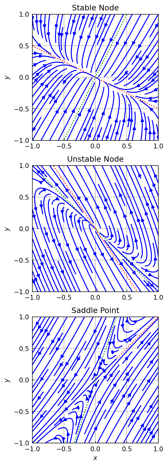
Both eigenvalues negative, \(\tau^2 -4\Delta > 0\), \(\tau<0\), \(\Delta>0\)
Stable Node: Since both eigenvalues are negative, it follows that \(\lim_{t \to \infty} \mathbf{x}(t)=\mathbf{0}\) in the direction of \(\mathbf{k}_1\) when \(c_1 \neq 0\) or in the direction of \(\mathbf{k}_2\) when \(c_1=0\)
Both eigenvalues positive, \(\tau^2 -4\Delta > 0\), \(\tau>0\), \(\Delta>0\)
Unstable Node:\(\mathbf{x}(t)\) becomes unbounded in the direction of \(\mathbf{k}_1\) when \(c_1 \neq 0\) or in the direction of \(\mathbf{k}_2\) when \(c_1=0\)
Eigenvalues have opposite signs, \(\tau^2 -4\Delta > 0\), \(\Delta<0\)
Saddle Point: When \(c_1=0\), \(\mathbf{x}(t)\) will approach \(\mathbf{0}\) along the line determined by \(\mathbf{k}_2\). If \(\mathbf{x}(0)\) does not lie on the line determined by \(\mathbf{k}_2\), the direction determined by \(\mathbf{k}_1\) serves as an asymtote for \(\mathbf{x}(t)\)
Example\(~\) Classify the critical point \((0,0)\) of each of the following linear system \(\mathbf{x}'=\mathbf{A}\mathbf{x}\) as either a stable node, an unstable node, or a saddle point
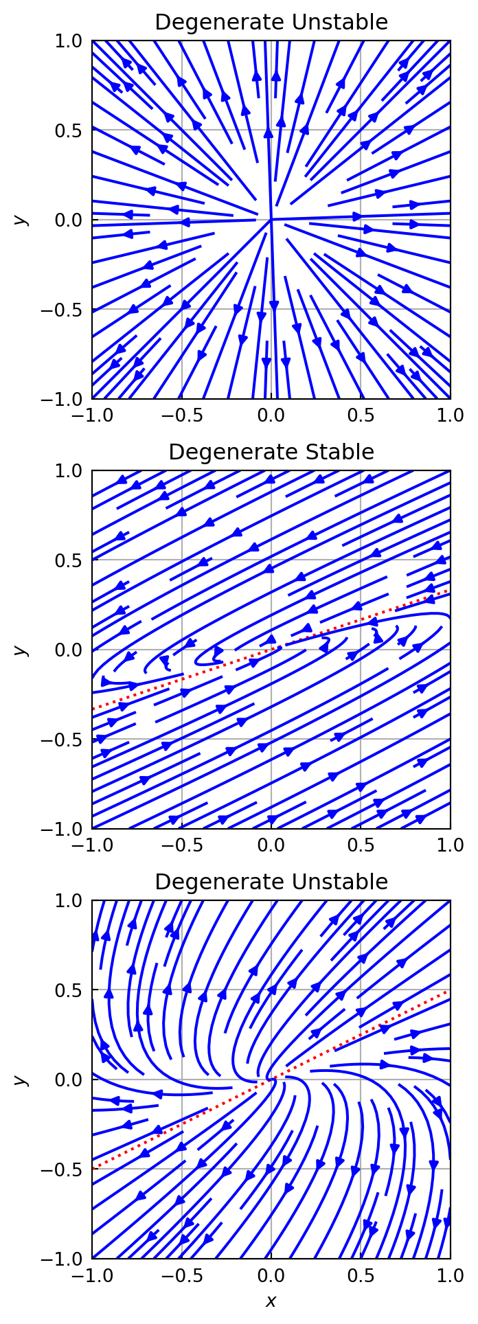
A Repeated Real Eigenvalue, \(\tau^2 -4\Delta = 0\)
The general solution takes on one of two different forms depending on whether one or two linearly independent eigenvectors can be found for the repeated eigenvalues \(\lambda_1\)
Two linearly independent eigenvectors
If \(\mathbf{k}_1\) and \(\mathbf{k}_2\) are two linearly independent eigenvectors corresponding to \(\lambda_1\), then the general solution is given by
If \(\lambda_1<0\), the \(\mathbf{x}(t)\) approaches \(\mathbf{0}\) along the line determined by the vector \(c_1\mathbf{k}_1 + c_2\mathbf{k}_2\) and the critical point is a degenerate stable node. The arrows are reversed when \(\lambda_1>0\), and the critical point is a degenerate unstable node
A single linearly independent eigenvectors
When only a single linearly independent eigenvector \(\mathbf{k}_{11}\) exists, the general solution is given by
where \((\mathbf{A} -\lambda_1\mathbf{I})\mathbf{k}_{12}=\mathbf{k}_{11}\). If \(\lambda_1<0\), then \(\lim_{t \to \infty} te^{\lambda_1 t}=0\) and it follows that \(\mathbf{x}(t)\) approaches \(\mathbf{0}\) in the line determined by \(\mathbf{k}_{11}\). The critical point is again a degenerate stable node. When \(\lambda_1>0\), \(\mathbf{x}(t)\) becomes unbounded as \(t\) increases, and the critical point is a degenerate unstable node
Example\(~\) Classify the critical point \((0,0)\) of each of the following linear system \(\mathbf{x}'=\mathbf{A}\mathbf{x}\)
If \(\lambda_1=\alpha +i\beta\) and \(\bar{\lambda}_1\) are the complex eigenvalues and \(\mathbf{k}_1=\mathbf{b}_1 +i\mathbf{b}_2\) is a complex eigenvector corresponding to \(\lambda_1\), the general solution can be written as \(\mathbf{x}=c_1\mathbf{x}_1 +c_2\mathbf{x}_2\)
\[
\begin{aligned}
\mathbf{x}_1(t) &=e^{\alpha t}\left(\mathbf{b}_1\cos\beta t -\mathbf{b}_2\sin\beta t\right) \\
\mathbf{x}_2(t) &=e^{\alpha t}\left(\mathbf{b}_2\cos\beta t +\mathbf{b}_1\sin\beta t\right)
\end{aligned}\]
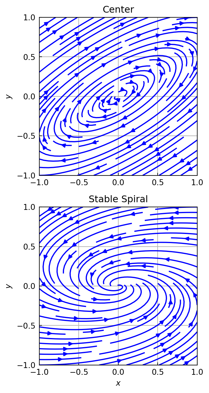
Pure imaginary roots, \(\tau^2 -4\Delta < 0\), \(~\tau=0\)
Center: When \(\alpha=0\), all solutions are ellipses with center at the origin and are periodic with period \(p=2\pi/\beta\). The critical point is called a center
Nonezero real part, \(\tau^2 -4\Delta < 0\), \(~\tau\neq 0\)
Spiral Point: When \(\alpha<0\), \(e^{\alpha t}\to 0\), and the elliptical-like solution spirals closer and closer to the origin. The critical point is called a stable spiral point. When \(\alpha>0\), the effect is the opposite. An elliptical-like solution is driven farther and farther from the origin, and the critical point is now called an unstable spiral point
Example\(~\) Classify the critical point \((0,0)\) of each of the following linear system \(\mathbf{x}'=\mathbf{A}\mathbf{x}\)
For a linear plane autonomous system \(\mathbf{x}'=\mathbf{A}\mathbf{x}\) with \(\mathrm{det}\,\mathbf{A}\neq 0\), let \(\mathbf{x}\) denote the solution that satisfies the initial condition \(\mathbf{x}(0)=\mathbf{x}_0\), where \(\mathbf{x}_0\neq\mathbf{0}\)
\(\lim_{t \to \infty}\mathbf{x}(t)=\mathbf{0}\) if and only if the eigenvalues of \(\mathbf{A}\) have negative real parts. This will occur when \(\Delta>0\) and \(\tau<0\)
\(\mathbf{x}(t)\) is periodic if and only if the eigenvalues of \(\mathbf{A}\) are pure imaginary. This will occur when \(\Delta>0\) and \(\tau=0\)
In all other cases, given any neighborhood of the origin, there is at least one \(\mathbf{x}_0\) in the neighborhood for which \(\mathbf{x}(t)\) becomes unbounded as \(t\) increases
8.3 Linearization and Local Stability
Here we will use linearization as a means of analyzing nonlinear DEs and nonlinear systems; the idea is to replace them by linear DEs and linear systems. Let \(\mathbf{x}_1\) be a critical point of an autonomous system, and let \(\mathbf{x}=\mathbf{x}(t)\) denote the solution that satisfies the initial condition \(\mathbf{x}(0)=\mathbf{x}_0\), where \(\mathbf{x}\neq\mathbf{x}_1\).
\(\mathbf{x}_1\) is a stable critical point
when, given any \(\rho > 0\), there is a \(r>0\) such that if \(\mathbf{x}_0\) satisfies \(|\mathbf{x}_0 -\mathbf{x}_1|<r\), then \(\mathbf{x}(t)\) satisfies \(|\mathbf{x}(t) -\mathbf{x}_1|<\rho\)\(\,\) for all \(t>0\). If, in addition, \(\lim_{t \to \infty} \mathbf{x}(t)=\mathbf{x}_1\) whenever \(|\mathbf{x}_0 -\mathbf{x}_1|<r\), we call \(\mathbf{x}_1\) an asymptotically stable critical point
\(\mathbf{x}_1\) is an unstable critical point
if there is \(\rho>0\) with the property that, for any \(r>0\), there is at least one \(\mathbf{x}_0\) that satisfies \(|\mathbf{x}_0 -\mathbf{x}_1|<r\), yet the corresponding solution \(\mathbf{x}(t)\) satisfies \(|\mathbf{x}(t) -\mathbf{x}_1|\geq\rho\)\(\,\) for at least one \(t>0\)
Example\(~\) Show that \((0,0)\) is a stable critical point of the nonlinear plane autonomous system
Using separation of variables, we see that the solution of the system is
\[ r=\frac{1}{t +c_1},\;\;\theta=t +c_2 \]
for \(r\neq 0\). If \(\mathbf{x}(0)=(r_0,\theta_0)\) is the initial condition in polar coordinates, then
\[ r=\frac{r_0}{r_0 t +1},\;\;\theta=t +\theta_0 \]
Note that \(r\leq r_0\)\(\,\) for \(t\geq 0\), and \(r\) approaches \(0\) as \(t\) increases. Therefore, given \(\rho>0\), a solution that starts less than \(\rho\) from the origin remains within \(\rho\) of the origin for all \(t\geq 0\). Hence the critical point \((0,0)\) is asymptotically stable
Example\(~\) When expressed in polar coordinates, a plane autonomous system takes the form
Show that \((x,y)=(0,0)\) is unstable critical point
We see that \(dr/dt=0\) when \(r=0\) and can conclude that \((x,y)=(0,0)\) is a critical point. \(~\) The differential equation can be solved using separation of variables. If \(r(0)=r_0\) and \(r_0\neq 0,\) then
it follows that no matter how close to \((0,0)\) a solution starts, the solution will leave a disk of radius \(\epsilon\) about the origin. Therefore \((0,0)\) is an unstable critical point
Linearization
We replace the term \(\mathbf{g}(\mathbf{x})\) in the original autonomous system \(\mathbf{x}'=\mathbf{g}(\mathbf{x})\) by a linear term \(\mathbf{A}(\mathbf{x} -\mathbf{x}_1)\) that most closely approximates \(\mathbf{g}(\mathbf{x})\) in a neighborhood of \(\mathbf{x}_1\). This replacement process is called linearization
When \(\mathbf{x}_1\) is a critical point of a plane autonomous system
The original system \(\mathbf{x}'=\mathbf{g}(\mathbf{x})\) may be approximated in a neighborhood of \(\mathbf{x}_1\) by the linear system \(\mathbf{x}'=\mathbf{A}(\mathbf{x} -\mathbf{x}_1)\), where
If the eigenvalues of \(\mathbf{A}=\mathbf{g}'(\mathbf{x}_1)\) have negative real part, then \(\mathbf{x}_1\) is an asymptotically stable critical point
If the eigenvalues of \(\mathbf{A}=\mathbf{g}'(\mathbf{x}_1)\) have positive real part, then \(\mathbf{x}_1\) is an unstable critical point
Example\(~\) Classify the criticl points of the following plane autonomous system
Since the determinant of \(\mathbf{A}_1\) is negative, \(\mathbf{A}_1\) has a positive real eigenvalue. Therefore \((\sqrt{2},2)\) is an unstable critical point. \(\mathbf{A}_2\) has a positive determinant and a negative trace, and so both eigenvalues have negative real parts. It follows that \((-\sqrt{2},2)\) is a stable critical point
Classifying Critical Points
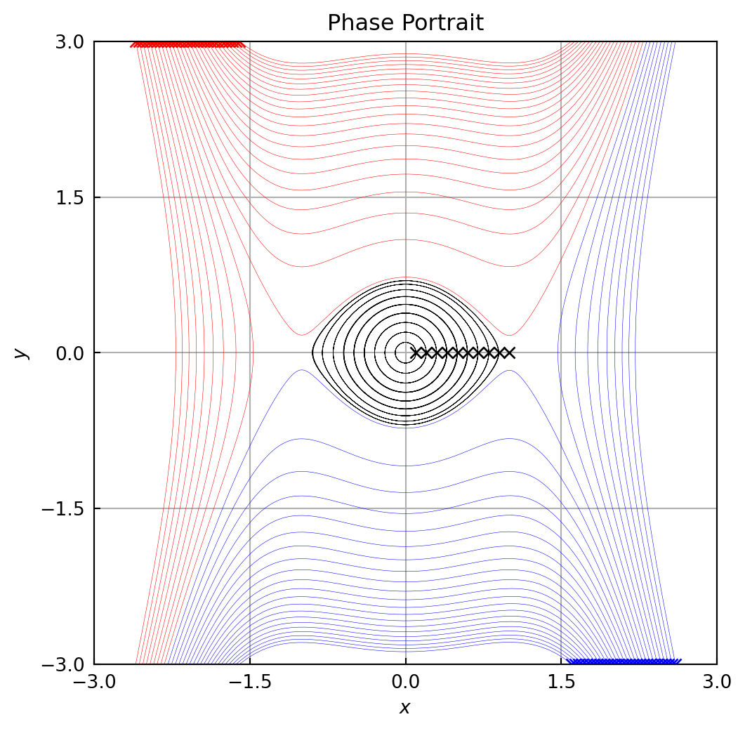
Example\(~\) The second-order differential equation \(mx'' +kx +k_1x^3 =0\), for \(k>0\), represents a general model for the free, undamped oscillations of a mass \(m\) attached to a nonlinear spring. If \(k=1\) and \(k_1=-1\), the spring is called soft and the plane autonomous system corresponding to the nonlinear second-order equation \(x'' +x -x^3=0\) is
Since \(\mathrm{det}\,\mathbf{A}_2<0\), critical points \((1,0)\) and \((-1,0)\) are both saddle points. The eigenvalues of \(\mathbf{A}_1\) are \(\pm i\), and the status of the critical points at \((0,0)\) remains in doubt. It may be either a stable spiral, an unstable spiral, or a center
Phase-Plane Method
The linearization method can provide useful information on the local behavior of solutions near critical points. It is of little help if we are interested in solutions whose initial condition \(\mathbf{x}(0)=\mathbf{x}_0\) is not close to a critical point or if we wish to obtain a global view of the family of solution curves. The phase-plane method is based on the fact that
and it attempts to find \(y\) as a function of \(x\) using one of the methods available for solving first-order DEs
Example\(~\) Use the phase-plane method to determine the nature of the solutions to \(x'' +x -x^3 =0\) in a neighborhood of \((0,0)\)
If we let \(dx/dt=y\), then \(dy/dt=x^3 -x\). From this we obtain the first-order DE
\[\frac{dy}{dx}=\frac{x^3 -x}{y} \]
which can be solved by separation of variables. Integrating gives
\[ y^2=\frac{x^4}{2}-x^2+c \]
If \(\mathbf{x}(0)=(x_0,0)\), where \(0<x_0<1\), then \(c=-\frac{x_0^4}{2} +x_0^2\), and so
\[ y^2=\frac{(2 -x^2 -x_0^2)(x_0^2 -x^2)}{2} \]
Note that \(y=0\) when \(x=-x_0\). In addition, the right-hand side is positive when \(-x_0<x<x_0\), and so each \(x\) has two corresponding values of \(y\). The solution \(\mathbf{x}(t)\) that satisfies \(\mathbf{x}(0)=(x_0,0)\) is therefore periodic, and so \((0,0)\) is a center
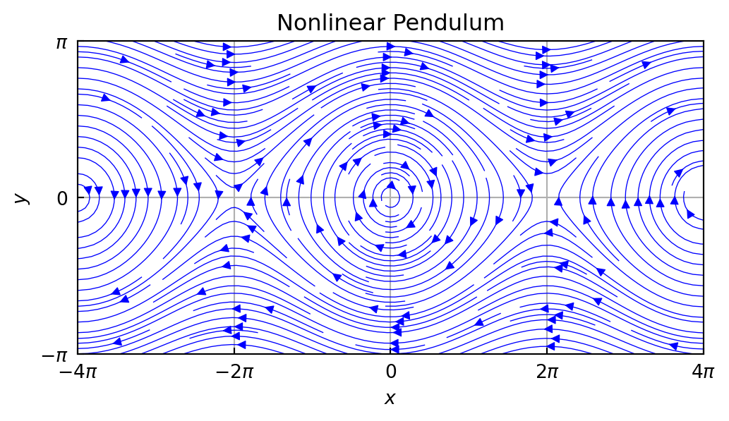
If \(k=2n+1\), \(\Delta<0\), and so all critical points \((\pm(2n+1)\pi,0)\) are saddle points. When \(k=2n\), the eigenvalues are pure imaginary, and so the nature of these critical points remains in doubt. From
Note that \(y=0\) when \(x=-x_0\), and that \((2g/l)(\cos x -\cos x_0)>0\) for \(|x|<|x_0|<\pi\). Thus each such \(x\) has two corresponding values of \(y\), and so the solution \(\mathbf{x}(t)\) that satisfies \(\mathbf{x}(0)=(x_0,0)\) is periodic. We may conclude that \((0,0)\) is a center. In the case of large initial velocities, the pendulum spins in complete circles about the pivot
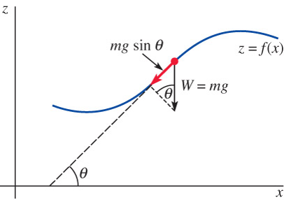
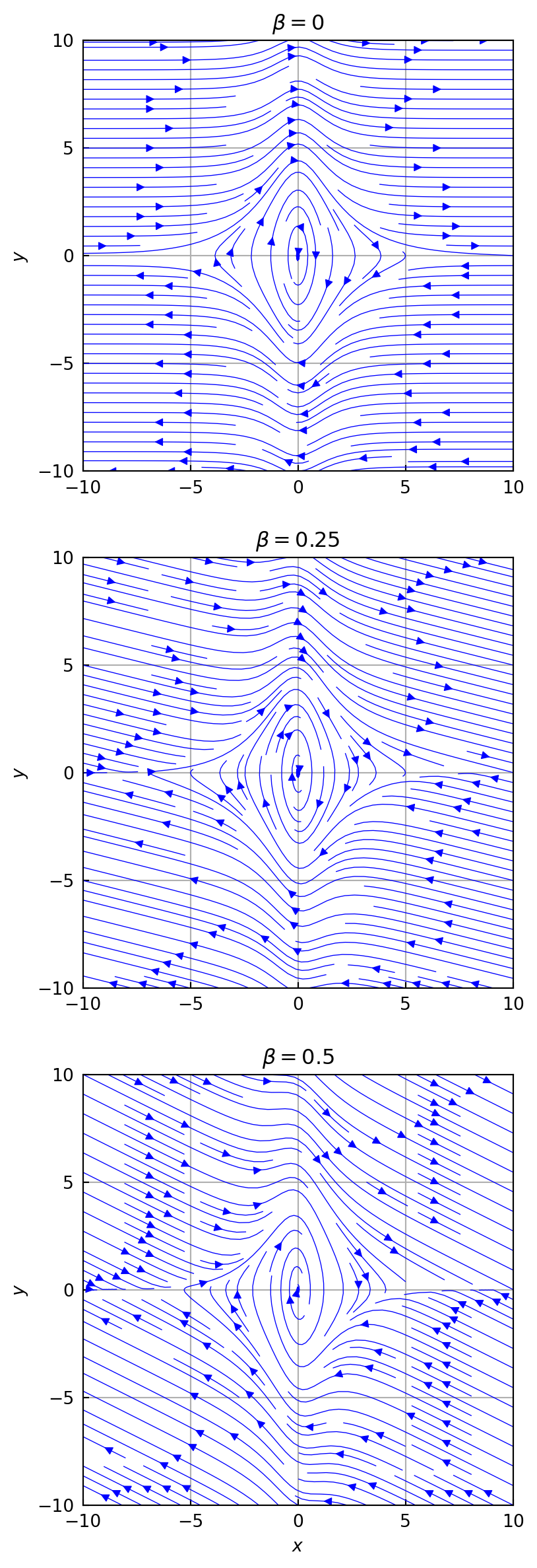
Suppose a bead with mass \(m\) slides along a thin wire whose shape is described by the function \(z=f(x)\). A wide variety of nonlinear oscillations can be obtained by changing the shape of the wire and by making different assumptions about the forces acting on the bead
The tangential force \(\mathbf{F}\) due to the weight \(W=mg\)\(\,\) has a magnitude \(mg\sin\theta\), and therefore the \(x\)-component of \(\mathbf{F}\) is \(F_x=-mg\sin\theta\cos\theta\). Since \(f'(x)=\tan\theta\), \(\,\) we can use the identity \(1+\tan^2\theta=\sec^2\theta\) to conclude that
A damping force \(\mathbf{D}\), in the direction opposite to the motion, is a constant multiple of the velocitcy of the bead. The \(x\)-component of \(\mathbf{D}\) is therefore
If \(\mathbf{x}_1=(x_1,y_1)\) is a critical point of the system, \(y_1=0\) and therefore \(f'(x_1)=0\). The bead must therefore be at rest at a point on the wire where the tangent line is horizontal. When \(f\) is twice differentiable, the Jacobian matrix at \(\mathbf{x}_1\) is
\(f''(x_1)<0\) : \(~\) A relative maximum therefore occurs at \(x=x_1\), and since \(\Delta<0\), \(\,\) an unstable saddle point occurs at \(\mathbf{x}_1=(x_1,0)\)
\(f''(x_1)>0\) and \(\beta>0\): \(~\) A relative maximum therefore occurs at \(x=x_1\), and since \(\tau<0\) and \(\Delta>0\), \(\,\mathbf{x}_1=(x_1,0)\) is a stable critical point.
If \(\beta^2 > 4gm^2f''(x_1)\), the system is overdamped and the critical point is a stable node. If \(\beta^2 < 4gm^2f''(x_1)\), the system is underdamped and the critical point is a stable spiral point. The exact nature of the stable critical point is still in doubt if \(\beta^2 = 4gm^2f''(x_1)\)
\(f''(x_1)>0\) and the system is undamped (\(\beta=0\)):
In this case the eigenvalues are pure imaginary, but the phase-plane method can be used to show that the critical point is a center. Therefore solutions with \(\mathbf{x}(0)=(x(0),x'(0))\) near \(\mathbf{x}_1=(x_1,0)\) are periodic
Example\(~\) A bead is released from the position \(x(0)=x_0\) on the curve \(z=\cosh(x)\) with initial velocity \(x'(0)=\nu_0\). Use the phase-plane method to show that the resulting solution is periodic when the system is undamped
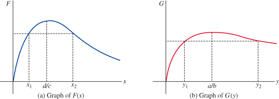
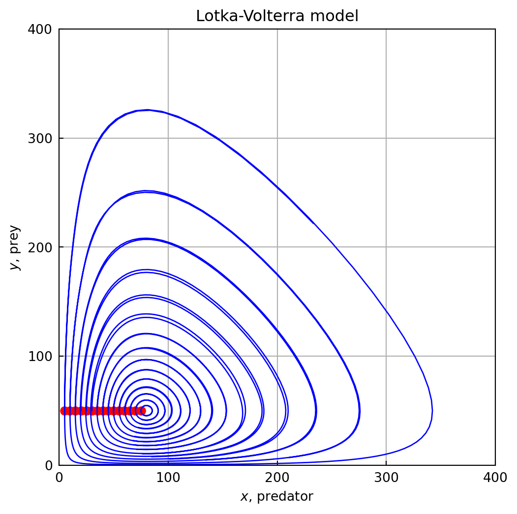
There are many predator-prey models that lead to plane autonomous systems with at least one periodic solution. The first such model was constructed independently by pioneer biomathematicians A. Lotka (1925) and V. Volterra (1926). If \(x\) denotes the number of predators and \(y\) denotes the number of prey, then the Lotka-Volterra model takes the form
where \(a\), \(b\), \(c\), and \(d\) are positive constants. The critical points of this plane autonomous system are \((0,0)\) and \((d/c,a/b)\), and the corresponding Jocobian matrices are
The critical point \((0,0)\) is a saddle point. Since \(\mathbf{A}_2\) has pure imaginary eigenvalues \(\lambda=\pm i\sqrt{ad}\), the critical point \((d/c,a/b)\) may be a center. This possibility can be investigated using the phase-plane method. Since
Typical graphs of the nonnegative functions \(F(x)=x^d e^{-cx}\) and \(G(y)=y^a e^{-by}\) are shown in
It is not hard to show that \(F(x)\) has an absolute maximum at \(x=d/c\), whereas \(G(y)\) has an absolute maximum at \(y=a/b\). These graphs can be used to establish the following properties of a solution curve that orginates at a noncritical point \((x_0,y_0)\) in the first quadrant
If \(y=a/b\), \(F(x)G(a/b)=c_0\) has two solutions \(x_m\) and \(x_M\) that satisfy \(x_m<d/c<x_M\)
If \(x_m<x_1<x_M\) and \(x=x_1\), \(\,\) then \(F(x_1)G(y)=c_0\) has exactly two solutions \(y_1\) and \(y_2\) that satisfy \(y_1<a/b<y_2\)
If \(x\) is outside the interval \([x_m,x_M]\), \(\,\) then \(F(x)G(y)=c_0\) has no solutions
Example\(~\) If we let \(a=0.1\), \(b=0.002\), \(c=0.0025\), and \(d=0.2\) in the Lotka-Volterra predator-prey model, the critical point in the first quadrant is \((d/c,a/b)=(80,50)\), and we know that this critical point is a center. The eigenvalues of \(\mathbf{g}'((80,50))\) are \(\lambda=\pm(\sqrt{2}/10)i\), and so the solutions near the critical point have period \(p\simeq 10\sqrt{2}\pi\)
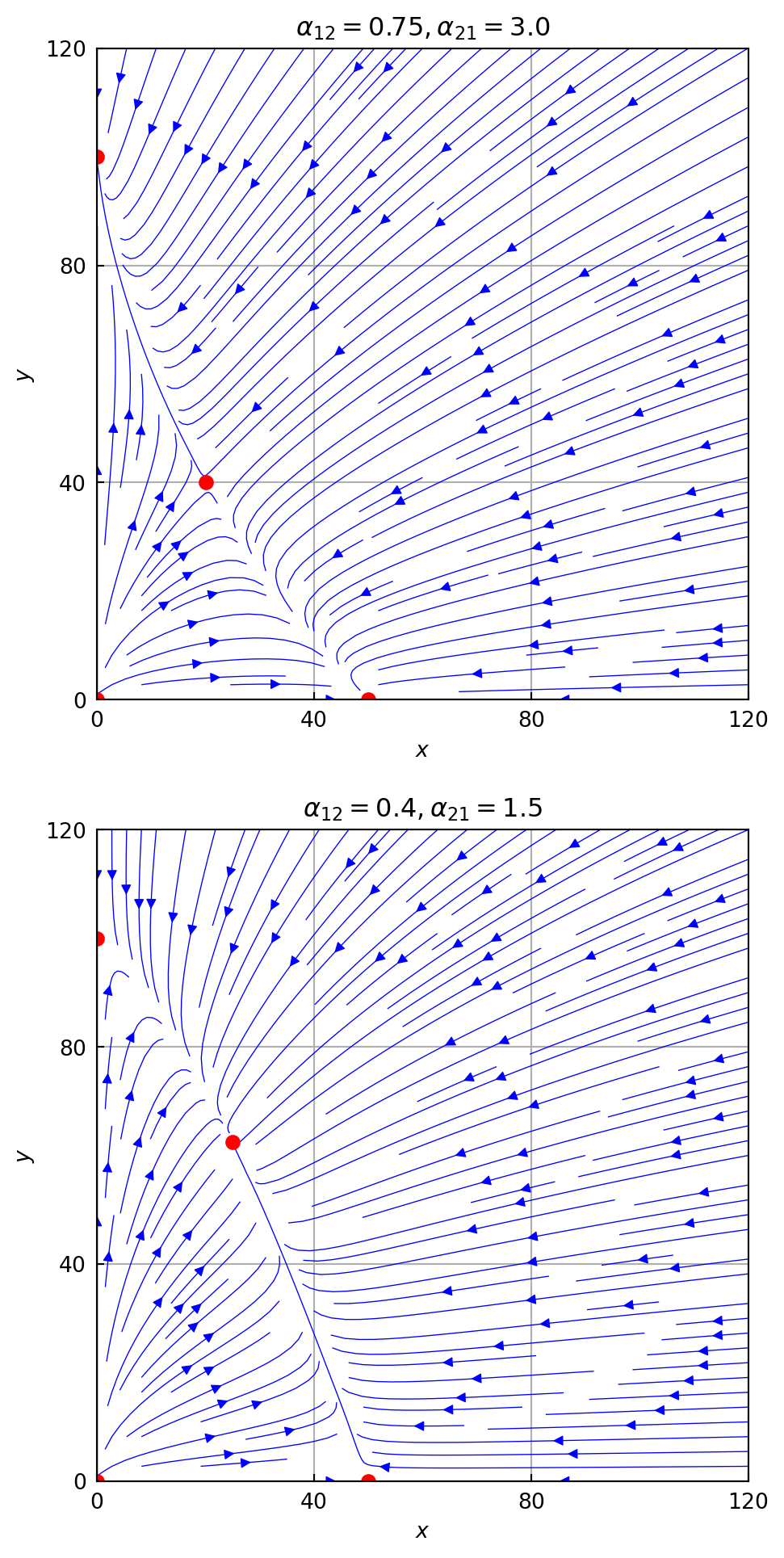
A competitive interaction occurs when two or more species compete for the food, water, light, and species resources of an ecosystem. A number of mathematical models have been constructed that offer insights into conditions that permit coexistence. If \(x\) denotes the number in species I and \(y\) denotes the number in species II, then the Lotka-Volterra model takes the form
Note that in the absence of species II (\(y=0\)), \(x'=(r_1/K_1)x(K_1 -x)\), and so the first population grows logistically and approaches the steady-state population \(K_1\). A similar statement holds for species II growing in the absence of speices I. The term \(-\alpha_{21}xy\) in the second equation stems from the competitive effect of species I on species II. The model therefore assumes that this rate of inhibition is directly proportional to the number of possible competitive pairs \(xy\) at a particular \(t\)
This plane autonomous system has critical points at \((0,0)\), \((K_1,0)\), and \((0,K_2)\). When \(\alpha_{12}\alpha_{21}\neq 0\), the lines \(K_1 -x -\alpha_{12}y=0\) and \(K_2 -y -\alpha_{21}x=0\) intersect to produce a fourth critical point \(\hat{\mathbf{x}}=(\hat{x},\hat{y})\)
8.5 Periodic Solutions, Limit Cycles, and Global Stability
In this section, we will investigate the existence of periodic solutions of nonlinear plane autonomous systems and introduce special periodic solutions called limit cycles
An analysis of critical points using linearization can provide valuable information on the behavior of solutions near critical points and insight into a variety of biological and physical phenomena. However there are some inherent limitations to this approach. When the eigenvalues of the Jacobian matrix are pure imaginary, we cannot conclude that there are periodic solutions near the critical point
The first goal of this section is to determine conditions under which we can either exclude the possibility of periodic solutions or assert their existence
A second goal is to determine conditions under which an asymptotically stable critical point is globally stable: \(\lim_{t \to \infty}\mathbf{x}(t)=\mathbf{x}_1\) for all initial conditions in a simply connected region \(\mathbb{R}\)
Negative Criteria
Theorem If a plane autonomous system has a periodic solution \(\mathbf{x}=\mathbf{x}(t)\) in a simply connected region \(\mathbb{R}\), then the system has at least one critical point inside the corresponding simple closed curve \(C\). If there is a single critical point inside \(C\), then that critical point cannot be a saddle point
Corollary If a simply connected region \(\mathbb{R}\) either contains no critical points of a plane autonomous system or contains a single saddle point, then there are no periodic solutions in \(\mathbb{R}\)
Example\(~\) Show that the Lotka-Volterra competition model
Another sometimes useful result can be formulated in terms of the divergence of the vector field
\[ \mathbf{v}(x,y)=\left(P(x,y), Q(x,y)\right) \]
Bendixson Negative Criterion
If \(\displaystyle\mathrm{div}\,\mathbf{v}=\frac{\partial P}{\partial x} +\frac{\partial Q}{\partial y}\) does not change sign in a simply connected region \(\mathbb{R}\), then the plane autonomous system has no periodic solutions in \(\mathbb{R}\)
Proof\(~\) Suppose, to the contrary, that there is a periodic solution \(\mathbf{x}=\mathbf{x}(t)\) in \(\mathbb{R}\), and let \(C\) be the resulting simple closed curve and \(R_1\) the region bounded by \(C\). By using Green’s theorem, we obtain
Since \(\displaystyle\mathrm{div}\,\mathbf{v}=\frac{\partial P}{\partial x} +\frac{\partial Q}{\partial y}\) is continuous and does not change sign in \(\mathbb{R}\), it follows that either \(\mathrm{det}\,\mathbf{v}\geq 0\) or \(\mathrm{det}\,\mathbf{v}\leq 0\) in \(\mathbb{R}\), and so
and so \(\displaystyle
\mathrm{div}\,\mathbf{v}=\frac{\partial P}{\partial x} +\frac{\partial Q}{\partial y}=-\frac{\beta}{m}<0\)
Dulac Negative Criterion
If \(\delta(x,y)\) has continuous first partial derivatives in a simply connected region \(\mathbb{R}\) and \(\displaystyle \frac{\partial (\delta P)}{\partial x} +\frac{\partial (\delta Q)}{\partial y}\) does not change sign in \(\mathbb{R}\), \(\,\) then the plane autonomous system has no periodic solutions in \(\mathbb{R}\)
Example\(~\) Use \(\delta(x,y)=1/(xy)\) to show that the Lotka-Volterra competition equations
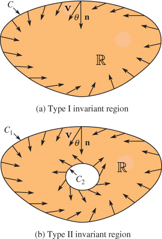
A region \(\mathbb{R}\) is called an invariant region for a plane autonomous system if, whenever \(\mathbf{x}_0\) is in \(\mathbb{R}\), the solution \(\mathbf{x}=\mathbf{x}(t)\) remains in \(\mathbb{R}\). If \(\mathbf{n}(x,y)\) denotes a normal vector on the boundary that points inside the region, then \(\mathbb{R}\) will be an invariant region for the plane autonomous system provided \(\mathbf{v}(x,y)\cdot\mathbf{n}(x,y)\geq 0\) for all points \((x,y)\) in the boundary
Poincaré-Benedixon I
Let \(\mathbb{R}\) be an invariant region for a plane autonomous system and suppose that \(\mathbb{R}\) has no critical points on its boundary
\((\text{a})\)\(~\) If \(\mathbb{R}\) is a type I region that has a single unstable node or an unstable spiral point in its interior, then there is at least one periodic solution in \(\mathbb{R}\)
\((\text{b})\)\(~\) If \(\mathbb{R}\) is a type II region that contains no critical points of the system, then there is at least one periodic solution in \(\mathbb{R}\)
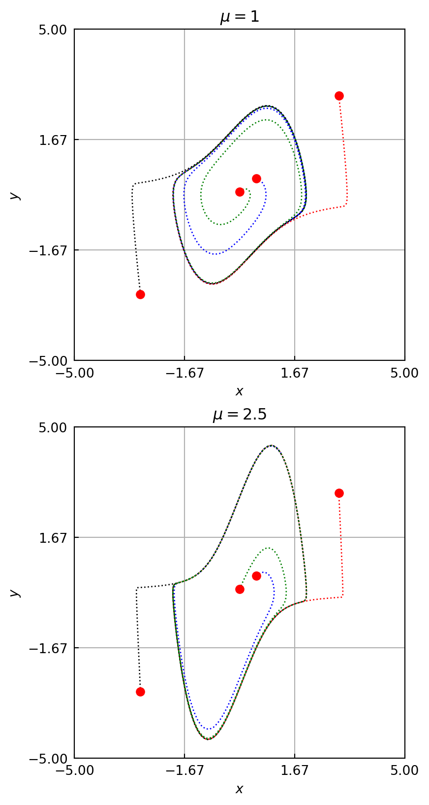
In either of the two cases, if \(\mathbf{x}=\mathbf{x}(0)\) is a nonperiodic solution in \(\mathbb{R}\), then \(\mathbf{x}(t)\) spirals toward a cycle that is a solution to the system. This periodic solution is called a limit cycle
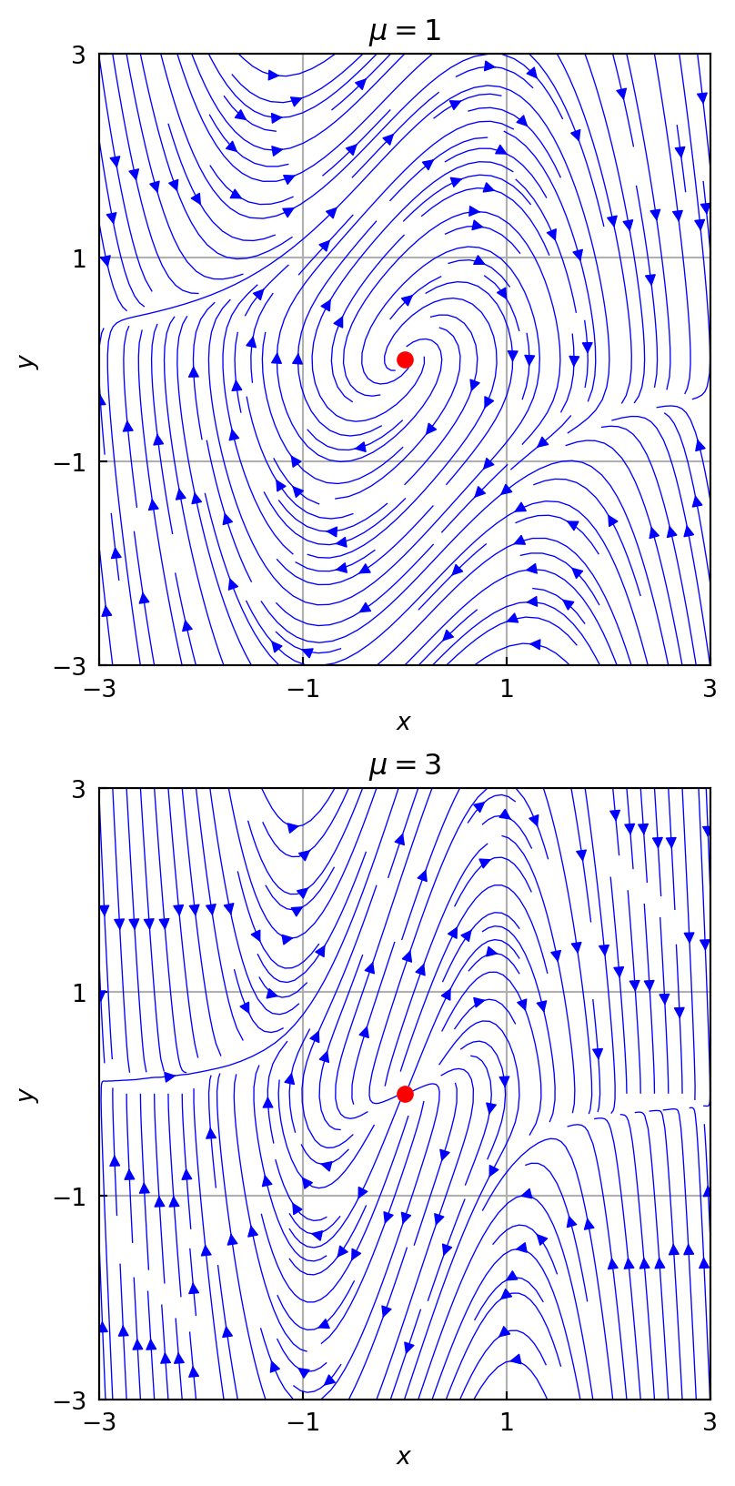
Example\(~\) The Van der Pol equation is a nonlinear second-order differential equation that arises in electronics, and as a plane autonomous system it takes the form
We will assumme that there is a Type I invariant region \(\mathbb{R}\) for the corresponding plane autonomous system and that this region contains \((0,0)\) in its interior. The only critical point is \((0,0)\), and the Jacobian matrix is given by
Therefore, \(\tau=\mu\), \(\Delta=1\), and \(\tau^2 -4\Delta=\mu^2-4\). Since \(\mu >0\), the critical point is either an unstable spiral point or an unstable node. By part (a) of Poincaré-Benedixon I, the system has at least one periodic solution in \(\mathbb{R}\)
Let \(\mathbb{R}\) be a type I invariant region for a plane autonomous system that has no periodic solutions in \(\mathbb{R}\)
\((\text{a})\)\(~\) If \(\mathbb{R}\) has a finite number of nodes or spiral points, then given any initial position \(\mathbf{x}_0\) in \(\mathbb{R}\), \(\lim_{t \to \infty} \mathbf{x}(t)=\mathbf{x}_1\) for some critical point \(\mathbf{x}_1\)
\((\text{b})\)\(~\) If \(\mathbb{R}\) has a single stable node or stable spiral point \(\mathbf{x}_1\) in its interior and no critical points on its boundary, then \(\lim_{t \to \infty} \mathbf{x}(t)=\mathbf{x}_1\) for all initial positions \(\mathbf{x}_0\) in \(\mathbb{R}\): globally stable
Example\(~\) Empirical evidence suggests that the plane autonomous system
has a type I invariant region \(\mathbb{R}\) that lies inside the reactangle defined by \(0\leq x \leq 2\), \(0 \leq y \leq 1\)
\((\text{a})\)\(~\) Use the Benedixson negative criterion to show that there are no periodic solutions in R
\((\text{b})\)\(~\) If \(\mathbf{x}_0\) is in \(\mathbb{R}\) and \(\mathbf{x}=\mathbf{x}(t)\) is the solution satisfying \(\mathbf{x}(t)=\mathbf{x}_0\), use Poincaré-Benedixon II to find \(\lim_{t \to \infty}\mathbf{x}(t)\)